Jaramillo et al. (2021b) | IH-MOOSE
Description
Shoreline evolution is a complex natural phenomenon involving longshore and cross-shore sediment transport, shoreline rotation, etc., which creates the need for hybrid models that simulate diverse situations. Jaramillo et al. (2021b) proposed a hybrid model for embayed beaches, IH-MOOSE (Model Of Shoreline Evolution), by integrating equilibrium-based cross-shore, planform, and rotation evolution models. In other words, IH-MOOSE combines the following models: (1) the equilibrium cross-shore evolution model (e.g. Yates et al., 2009), (2) the equilibrium planform model (e.g.Hsu and Evans, 1989), and (3) the equilibrium shoreline rotation model (e.g. Jaramillo et al., 2021a). With few calibration parameters required, IH-MOOSE is a reduced-complexity model compared to the other process-based models.
While any combination of cross-shore EBSEM, beach planform, and rotational EBSEM can be applied in this methodology, the hybrid model suggested by Jaramillo et al. (2021) originally combined the following three models:
(1) Equilibrium cross-shore evolution model (Yates et al., 2009):
\(E\) : the incoming breaking wave energy related to the breaking wave height (water depth at breaking \(h_b\) and breaking index γ) as \(E=(\frac{H_b}{4.004})^2=(\frac{γ}{4.004})^2 h_b^2\)
\(E_{eq}\) : the equilibrium wave energy corresponding to the current shoreline position
\(S(t)\) : the shoreline position at time \(t\)
\(S_{eq}\) : the equilibrium shoreline position
\(C^±\) : the free parameters where \(C^+\) indicates the accretion and \(C^-\) indicates the erosion, respectively
(2) Equilibrium planform model (Hsu and Evans, 1989):
\(R\) : the radius measured from the tip of the headland breakwater
\(R_o\) : the length of the control line joining the updrift diffraction point to the down-coast control point
\(θ\) : the angle between the location of \(R\) on the shoreline
\(β\) : the angle between the control line and the wavefront at the diffraction point
\(C_i\) : the calibration parameters that depend on the wave obliquity (\(β\)) based on measured shapes of the model beaches (\(i\)=0,1 and 2)
(3) Equilibrium shoreline rotation model (Jaramillo et al., 2021)
Jaramillo et al. (2021) suggested a shoreline rotation model that predicts the temporal evolution of the shoreline orientation based on the concept of previous research and the observation data as follows:
\(P\) : the incoming wave power related to the significant wave height \(H_s\) and the wave peak period \(T_p\) as \(P=H_s^2T_p\)
\(α_{s,eq}\) : the asymptotical equilibrium shoreline orientation
\(α_s(t)\) : the shoreline orientation at time \(t\)
\(L^±\) : the proportional constants where \(L^+\) indicates the clockwise shoreline rotation and \(L^-\) indicates the counterclockwise rotation, respectively
Fig. 3-5-1 shows the definition sketch of hybrid shoreline evolution model proposed by Jaramillo et al. (2021b). Here, the equilibrium planform is rotated and retreated from the pivot point to predict the shoreline.
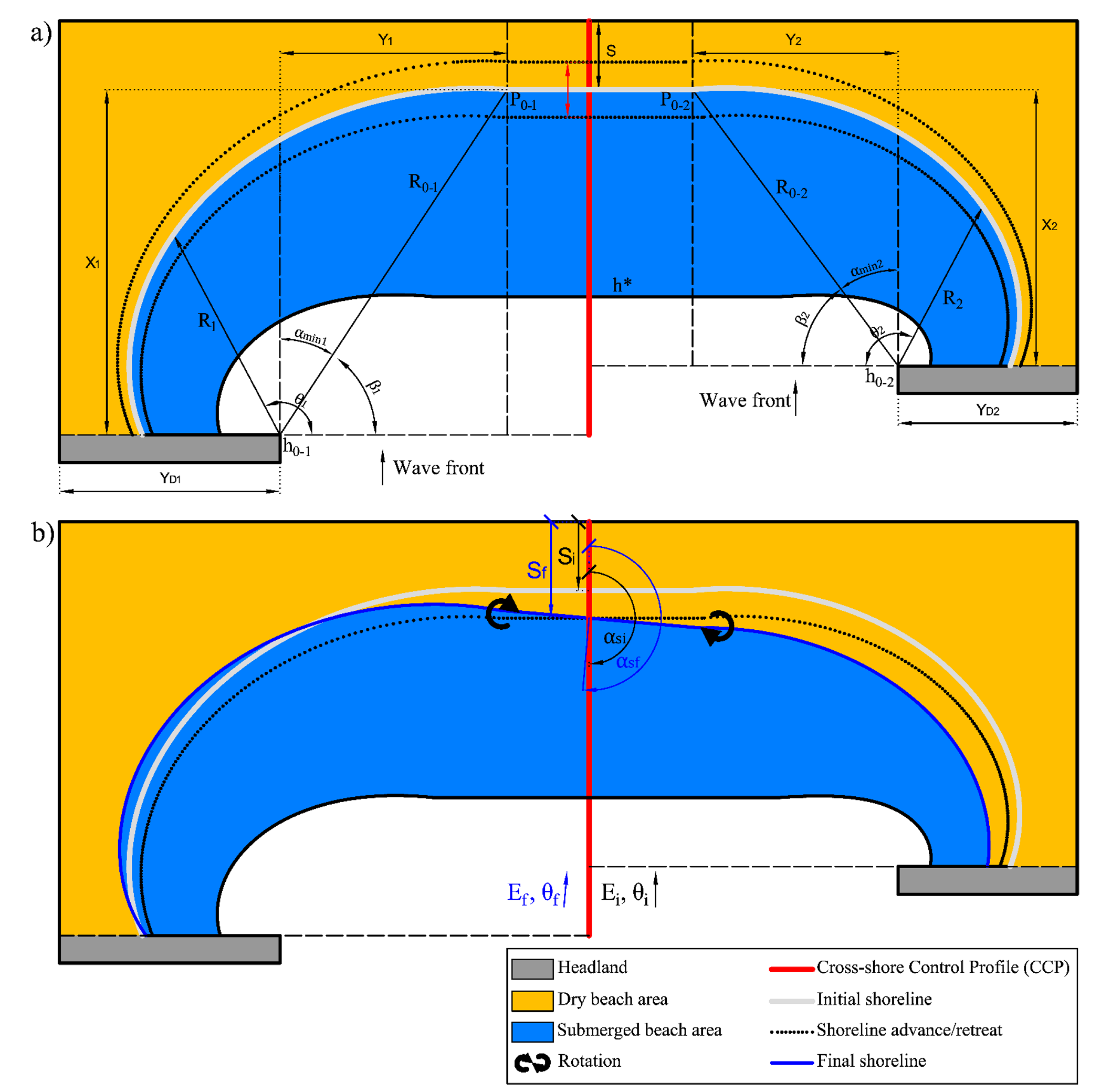
Fig. 3-5-1. Definition sketch of hybrid shoreline evolution model proposed by Jaramillo et al. (2021b).
Simulation procedure
The following describes the procedure for simulating the Jaramillo et al. (2021b) model. The figure below (Fig. 3-5-2) illustrates the start screen for simulating the model.
Upload the required file (see NetCDF file in Simulation inputs below) using the Browse File button in the Models tab.
Select the desired model from the list of modules to open the model’s start screen.
Adjust the input parameters and simulation settings in the side panel according to the model’s requirements (see Simulation settings below).
Click on the “Run Model” button to start the model execution.
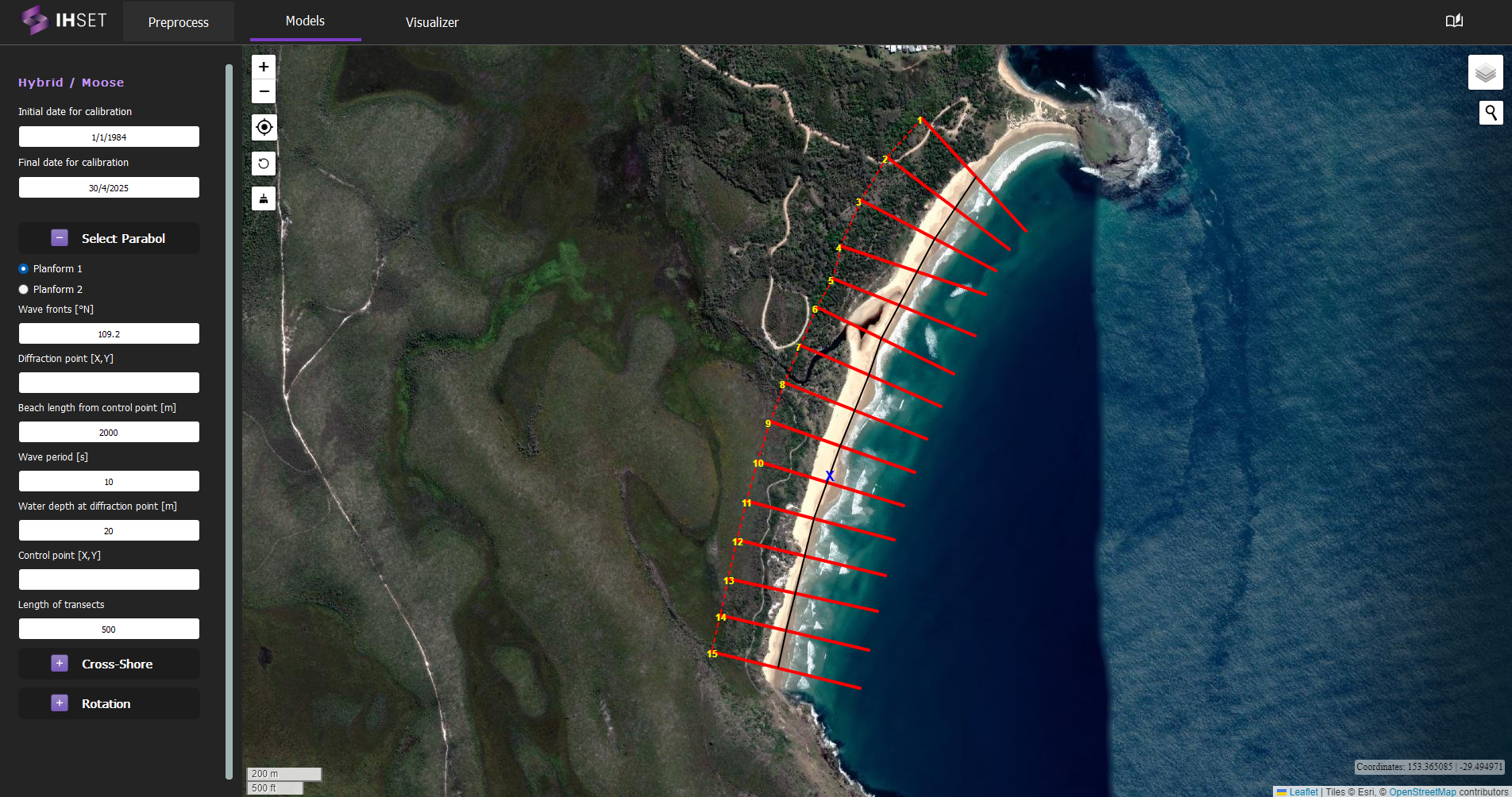 Fig. 3-5-2. Start screen for simulating IH-MOOSE at Angourie Back Beach, Australia.
Simulation settings
For equilibrium cross-shore evolution model The user can choose the model to predict cross-shore evolution. For more information on the simulation settings, please refer to the links for each of the models below.
Yates et al. (2009) - Original IH-MOOSE
For equilibrium planform model The user can choose the model to predict the equilibrium planform model. For more information on the simulation settings, please refer to the links for each of the models below.
Hsu and Evans (1989) - Original IH-MOOSE
For equilibrium shoreline rotation model The user can choose the model to predict longshore evolution. For more information on the simulation settings, please refer to the links for each of the models below.
Jaramillo et al. (2021a) - Original IH-MOOSE
Additional simulation settings
Num parabolics : Number of parabolic equilibrium planform (one or two)
Simulate profiles : Choose profiles to simulate IH-MOOSE
Pivot profile : Choose reference profile to pivot the planform. IH-SET recommends that users select the profile in the center.
Simulation results
Using the dataset provided along with the IH-SET software for Angourie Back Beach, Australia, running the model simulation yields several outputs as shown in Fig. 3-5-3:
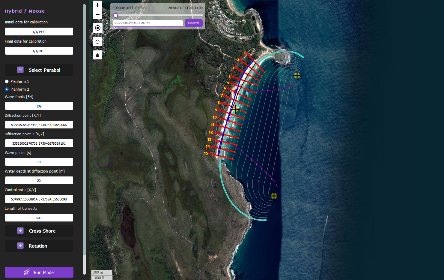 Fig. 3-5-3. Results of simulating IH-MOOSE for Angourie Back Beach, Australia using Yates et al. (2009), Jaramillo et al. (2021a), and the planform settings shown.
The primary output of this model is the shoreline position at that time \((t,S(t))\) for each profile data. The following options allow for proper viewing and analysis of these results:
Map View: All results are plotted over the same map view shown in Fig. 3-5-3 for easy visualization.
Clickable Transects: Plotted in red, the transects can be individually selected to view the shoreline observations and model results along the transect in plot form. Similar to the other plots generated by IH-SET, the toolbar options can be used to modify and save these plots.
Shoreline Position: Plotted in blue, this line connects the calculated shoreline position at each transect for the selected time stamp to represent the modeled shoreline location.
Adjustable Date-Time: Using the slider or the search bar in the top left, the user can select the time stamp for which the shoreline position is displayed on the map.