Turki et al. (2013)
Description
Turki et al. (2013) proposed a model based on the same differential equation governing the exponential beach response used in Miller and Dean (2004). To apply this differential equation, the study assumed that beach rotation is independent of other movements, such as cross-shore beach migration and beach breathing, and instead depends on the power and direction of incident waves. This model also works under the assumption that wave conditions remain steady and that the long-term equilibrium shoreline position affects how the shoreline changes in the short term. These assumptions led to the development of a shoreline rotation model in which the shoreline response rate is expressed as proportional to the difference between the instantaneous position (\(R(t)\)) and the equilibrium rotation (\(R_∞\)) as follows (Fig. 3-3-2-1-1):
\(ω\) : the ratio of beach change which is proportional to the characteristic time scale \(T_s\) (\(ω=1/T_s\))
\(R_∞\) : the equilibrium shoreline response
\(R(t)\) : the instantaneous position at time \(t\)
\(R_∞\) and \(R(t)\) can be calculated geometrically as a function of the beach length l as below:
\(β\) : the angle between the initial shoreline position and the wave crest
\(α(t)\) : the shoreline rotation angle at time \(t\)
The characteristic time scale \(T_s\) is inversely proportional to the beach change rate and governs the time it takes for the shoreline to reach a new equilibrium shoreline under new forcing conditions. According to the volumetric change based on the alongshore sediment transport, \(T_s\) is calculated as follows:
\(l\) : the beach length
\(K\) : the transport coefficient which is related to sediment characteristics such as sediment density \(ρ_s\), water density \(ρ_w\), gravity acceleration \(g\), sediment porosity a and dimensionless proportionality coefficient \(k\)
\(F_r\) : the energy flux per unit required to move sediments
\(h*\) : the closure depth which is expressed as the function of the wave height \(H_s\), where \(C_c\) is a constant value that differs from one beach to another
\(x(β,R(t))\) : the coefficient which is defined as follows:
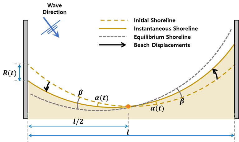
Fig. 3-3-2-1-1. Definition sketch of shoreline rotation model proposed by Turki et al. (2013).
The model proposed by Turki et al. (2013) was deliberately created to be simple, excluding a calibration factor to remain computationally efficient. However, several hypotheses were applied in developing the model that may limit its applicability to other beaches, such as the assumption of a linear shoreline and constant beach profile. Nonetheless, the model can be reliably applied to short, microtidal pocket beaches to reflect temporal patterns and variations in the medium to long term.
Simulation procedure
The following describes the procedure for simulating the Turki et al. (2013) model. The figure below illustrates the start screen for simulating the model.
Upload the required file (see NetCDF file in Simulation inputs below) using the Browse File button in the Models tab.
Select the desired model from the list of modules to open the model’s start screen.
Adjust the input parameters and simulation settings in the side panel according to the model’s requirements (see Calibration settings in Simulation inputs below).
Click on the “Run Model” button to start the model execution.
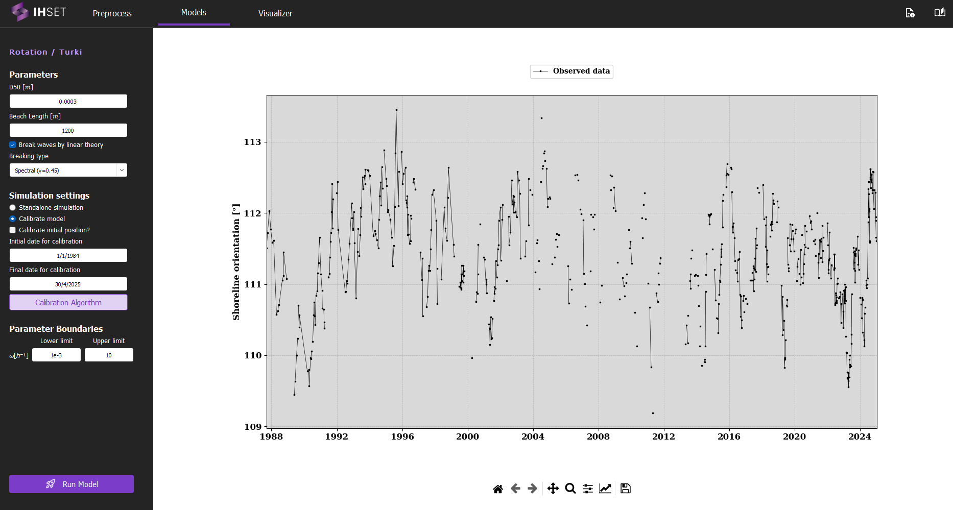
Fig. 3-3-2-1-2. Start screen for simulating the Turki et al. (2013) model.
Simulation inputs
This section outlines the input file, parameters, and simulation settings necessary to run this model in accordance with the procedure provided in the previous section.
NetCDF file
The primary input to run the Turki et al. (2913) model is the NetCDF file produced using the Preprocess module. More information about the contents of this dataset can be found here. This file provides the wave forcing data, comprised of wave data, optional sea level data, and the calculated bathymetry angle, which are inputted directly into the equations for the model. The NetCDF also contains the shoreline observation data, which are used to calibrate the model. For more information about the calibration process and parameters, please check the Calibration section.
As mentioned in the Simulation Procedure, this file is inputted in the Module tab prior to selecting the model. Once the required data for simulation is added and the model is selected, the screen transitions to the view shown in Fig. 3-3-2-1-2 above.
Parameters
In addition to the NetCDF file provided, a number of parameters must be entered into the module on the left side of the interface. These parameters are assumed to be constant over time and are included as constants in this model as follows:
D50 \([m]\) : Median grain size (Range : [0 ~ 2.0e-3])
Beach Length \([m]\) : Beach Length (Range : [0 ~ 3600.0])
Note that the Turki et al. (2013) model is especially sensitive to the Beach Length parameter, so it is important that this value be entered accurately for strong results.
If “Break waves by linear theory” is selected, the user will have the option to select the Breaking type (spectral or monochromatic), which determines the breaker index (\(γ\)) used.
Calibration Settings
Finally, the simulation settings and parameter boundaries must be selected for calibration. In the side panel, the user can decide to run a standalone simulation or to calibrate the model, described as follows:
Standalone simulation: The model is run with no calibration required, as the date range and parameter values will be entered manually. The option to use the first observation as the initial shoreline position (\(a_0\)) or to enter it manually will also be given.
Calibrate model: As opposed to the standalone simulation, this will run the model with calibration. The user can then decide whether or not to calibrate the initial position, \(α_0\).
When calibrating the model, the default initial and final dates for calibration will coincide with the start of the wave data and the end of the shoreline data respectively, though these values can be modified to better suit the data used and the desired output. It is important to note that that results for the Turki et al. (2013) model will require a warm-up period to calibrate and apply the bias of the free parameters correctly. For this reason, it is necessary to select a calibration parameter that considers bias, such as MSS, and that calibration begin a couple years before the shoreline observations for accurate results.
The user also has the option to modify the calibration algorithm and the parameter boundaries. Though it is not necessary to modify these elements, doing so may can improve the performance or run time of the model.
Simulation results
Using the dataset provided along with the IH-SET software for Angourie Back Beach, Australia, running the model simulation yields several detailed outputs as shown in Fig. 3-3-2-1-3:
Comparison of Model Simulation Results and Observed Data: This shows the differences between the model’s orientation predictions and actual observed data over the simulation period.
Time-Series Variation of Forcing Variables: Displays changes in key forcing variables, such as wave climate and sediment transport, over time, providing context for the orientation response.
Parameter Table Using Calibration Algorithm: Lists the parameters optimized for the model simulation, which are derived from calibration processes to enhance model accuracy.
Calibration and Validation Metrics: A table summarizing performance indicators such as RMSE (Root Mean Square Error), NS (Nash-Sutcliffe Efficiency), R² (Coefficient of Determination), and Bias, assessing the model’s predictive accuracy during both calibration and validation phases.
These outputs together provide a comprehensive view of model performance and reliability, allowing users to evaluate and interpret the shoreline evolution predicted by the simulation.
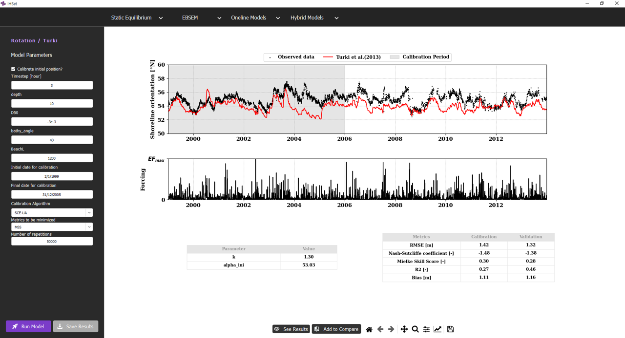
Fig. 3-3-2-1-3. Simulation results for Turki et al. (2013).
In addition, several other functionalities enhance the usability of the model simulation interface:
“Save Results” Button: Allows users to save the simulation results to an output NetCDF file, enabling further analysis or documentation of the model output. All saved simulations can be viewed in the “Visualizer” to compare the results with other EBSEM models, facilitating a side-by-side evaluation of model performance. For more details, please check Visualizer
Other buttons: These buttons allow users to customize and adjust the figures related to the simulation results. Users can modify visual elements such as axis labels, graph types, or legends for clearer interpretation or presentation. Once the desired adjustments are made, users can save the figures in various formats for further use or reporting.
These features enable users not only to analyze and retain results but also to compare multiple models effectively for enhanced decision-making in shoreline evolution modeling.