Bernabeu et al. (2003)
Description
Bernabeu et al. (2003) proposed an equilibrium beach profile (EBP) that aimed to improve representations of profile morphology and its seasonal variations more accurately by taking into account the influence of wave reflection. The resulting two-section EBP (2S-EBP) predicts the static beach profile for two separated sections (i.e., surf and shoaling profiles) as follows (Fig. 3-2-1-2-1):
Surf profile:
Shoaling profile:
\(h\) : the water depth from the mean sea level
\(x\) : the cross-shore distance from the shoreline
\(A,B,C,D\) : the calibration parameters that depend on the energy dissipation (i.e., \(A\) for the surf profile and \(B\) for the shoaling profile) and the reflection process (i.e., \(C\) for surf profile and \(D\) for shoaling profile)
\(x_0\) : the cross-shore distance between the beginning of the surf profile and the virtual origin of the shoaling profile over the mean sea level. The cross-shore distance \(x_0\) can be expressed as follows:
Here, \(h_r\) is the discontinuity point of water depth from the mean sea level.
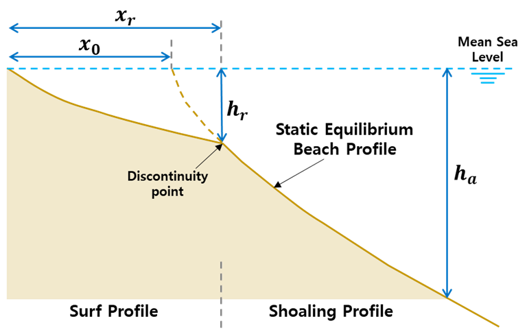
Fig. 3-2-1-2-1. Definition sketch of 2 section equilibrium beach profile model.
The given expression for the surf profile assumes that energy dissipation per unit volume is constant and that the relationship between wave height and depth is constant. It is the sum of two terms, the first based on the Dean (1977) profile and the second accounting for wave reflection. The profile beyond the surf zone is the shoaling profile, which is defined assuming that bottom friction dissipation per unit area is constant. The resulting expression is similar to that for the surf profile but is displaced by the length of the surf profile.
Simulation procedure
The following describes the procedure for simulating the Bernabeu et al. (2003) model. The figure below illustrates the start screen for simulating the model.
Upload the files needed by the model in the section below (Please see Inputs in Simulation settings)
Adjust the input parameters in the side panel according to the model’s requirements (Please see Parameters & Calibration settings in Simulation settings)
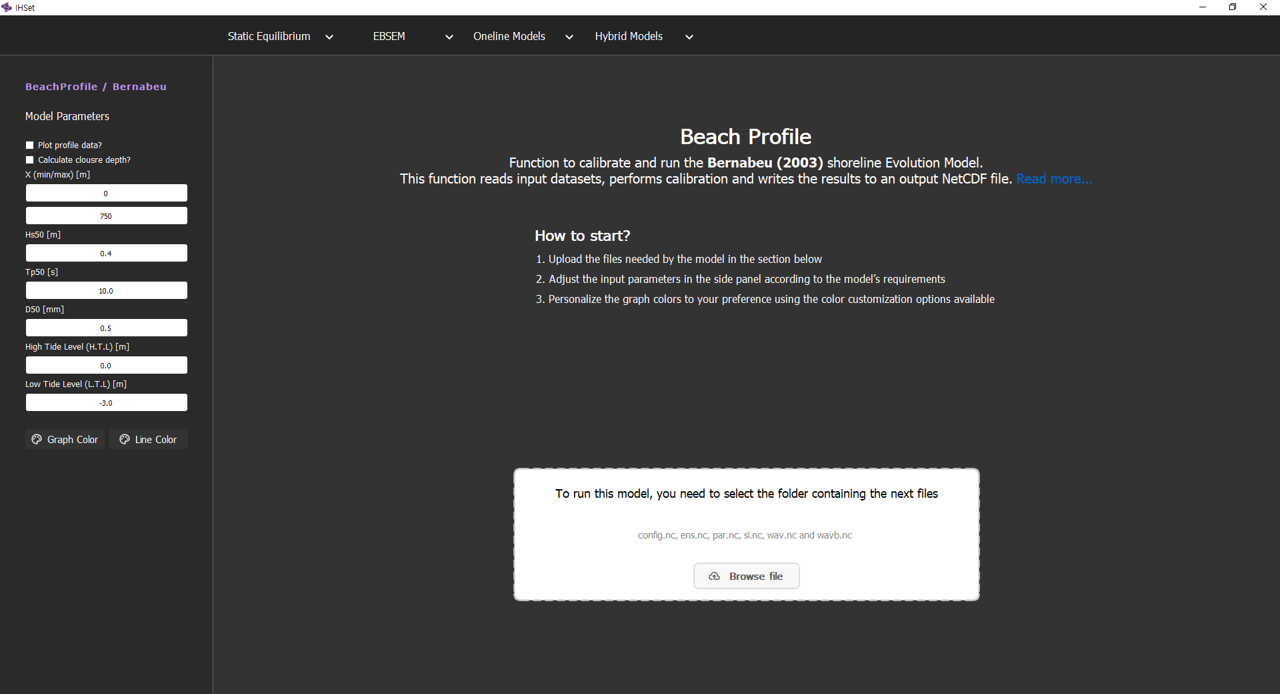
Fig. 3-2-1-2-2. Start screen for simulating the Bernabeu et al. (2003) model.
Simulation settings
Dataset (CSV/netCDF)
Dataset for calculating closure depth
wav.nc (optional)
Time : the time variation presented with the year [YYYY], month [MM], day [DD], and hour [hh]
\(H_s\) : the significant wave height to calculate breaking wave height \([m]\)
\(T_p\) : the peak wave period to calculate breaking wave height \([sec]\)
Dataset for plotting observation
prof.csv (optional)
x : the offshore distance from shoreline \([m]\)
z : the water depth according to the offshore distance \([m]\)
By clicking the “Browse file” button (see Fig. 3-2-1-2-2), you can select a folder containing the plotted dataset, allowing you to load the optional NetCDF/CSV files.
For more details, please check Preprocessed dataset
Parameters
X (min/max) : Range of cross-shore distance to calculate equilibrium profile \([m]\) (Range : [0 ~ 1500])
Hs50 : Significant wave height to calculate the dimensionless fall velocity \([m]\) (Range : [0 ~ 5.0])
Tp50 : Peak wave period to calculate the dimensionless fall velocity \([s]\) (Range : [0 ~ 20.0])
D50 : Median grain size \([mm]\) (Range : [0 ~ 2.0])
High Tide Level (H.T.L) : High Tide Level \([m]\) (Range : [L.T.L ~ 5.0])
Low Tide Level (L.T.L) : High Tide Level \([m]\) (Range : [-5.0 ~ H.T.L])
Calibration settings
Plot profile data? : Select whether to plot profile data together. To plot profile data, you need to have observed profile data \((x, h)\).
Calculate closure depth? : Select whether to calculate the closure depth. To calculate the closure depth, you need to have wave climate data \((H_s, T_p)\).
Simulation results
Running the model simulation yields several detailed outputs as shown in Fig. 3-2-1-2-3. Buttons in the display allow users to customize and adjust the figures related to the simulation results. Users can modify visual elements such as axis labels, graph types, or legends for clearer interpretation or presentation. Once the desired adjustments are made, users can save the figures in various formats for further use or reporting.
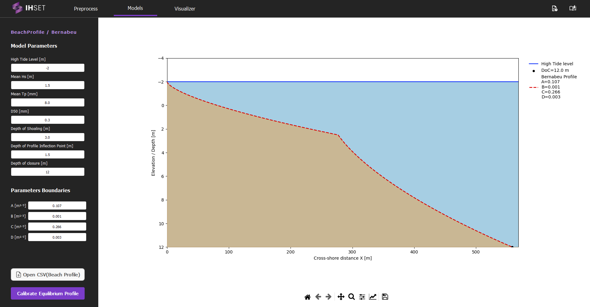
Fig. 3-2-1-2-3. Simulation results according to the settings for Bernabeu et al. (2003).
Calibration of the Bernabeu profile with field data.
For the calibration of the Bernabeu model, a beach profile measured in the field with X,Y input data can be used, where X is the distance of the profile perpendicular to the coastline and Z is the vertical variation of the profile from the zero reference point.
The example below shows the input CSV file format for the Bernabeu model for calibration with field profile data, where it is important to highlight the presence of the X,Y header for the correct loading of data when using the button: “Open CSV (Beach Profile)”:
X,Y
0.0,-5.8508468
1.0137528294529534,-5.80088
2.027505658905907,-5.7509133
3.04125848835886,-5.7009465
4.055011317811814,-5.6521598
5.068764147264767,-5.602193
6.08251697671772,-5.5522262
7.096269806170674,-5.5022595
8.110022635623627,-5.4522927
9.12377546507658,-5.4023259
10.137528294529535,-5.3535392
...
452.1337619360172,12.995833
453.1475147654702,13.101818
454.1612675949231,13.231795
Note: The high tide level (HTL), depth of closure (DoC), shoaling depth, and profile inflection depth data can be adjusted in the model parameters, and a new recalibration of the loaded profile may be requested.
Example dataset for calibration (Download)
An example beach profile dataset compatible with the Bernabeu et al. (2003) calibration workflow is available for download below.
Download example ZIP:
sha256:e56b5fd740e8c5bd44487d4a407392f676139e34571c9f6be054c98bae1c42aa
Calibration is performed using the least squares method by approximation along the X-axis (Figure 3-2-1-2-3).
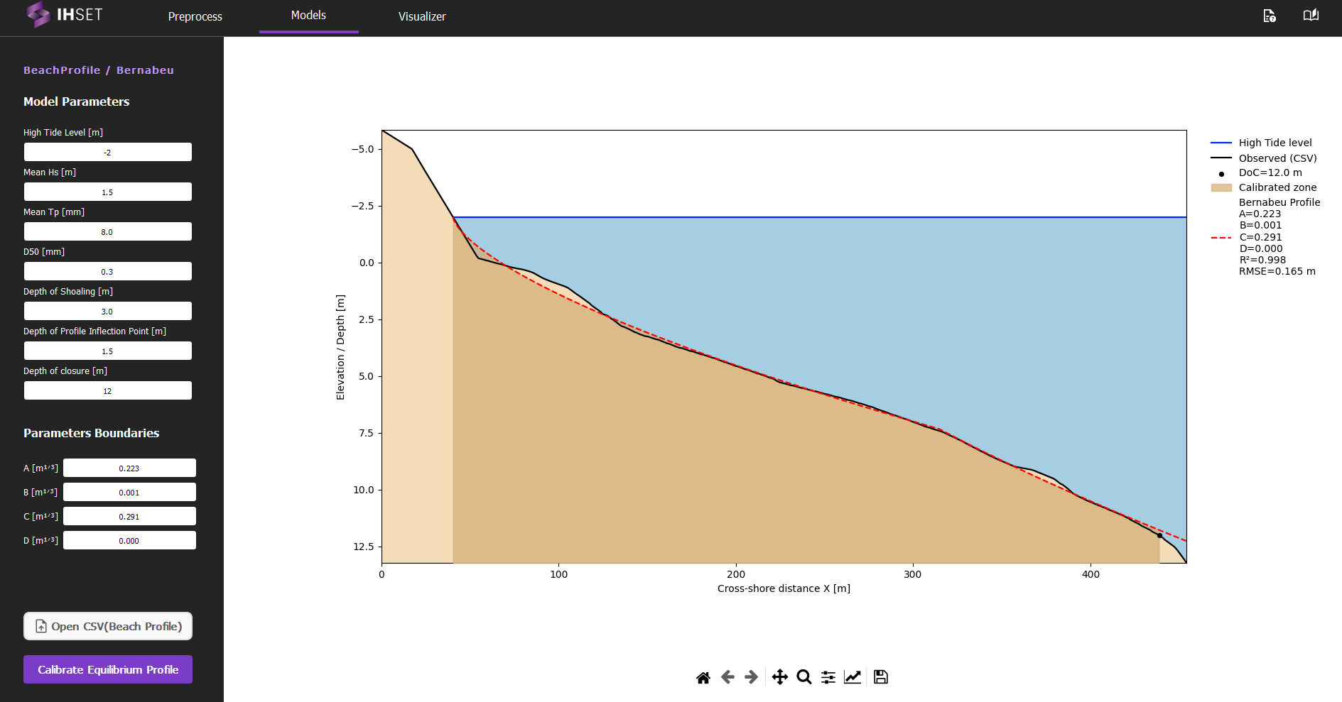
Fig. 3-2-1-2-3. Simulation results according to the settings for Bernabeu et al. (2003), using a CSV from surveyed beach profile to calibrate the model.