Lim et al. (2022)
Description
Lim et al. (2022) derived the shoreline evolution model based on the concept of horizontal behavior of suspended sediment. This study follows the assumptions made by Dean (1973) and Wang et al. (1975) that the dominant mode of cross-shore transport is suspension, the rate of which is governed by the dimensionless settling velocity and associated with energy dissipation across the shore. Applying the equations for these physical phenomena, Lim et al. (2022) proposed an ordinary differential equation (ODE) model as follows:
\(S(t)\) : the shoreline position at time \(t\)
\(E_b\) : the incident wave energy
\(k_r,a_r\) : the beach recovery and response factors
In addition, Lim et al. (2022) takes into account the effect of wave setup to improve model performance, especially during storm events, as follows:
\(H_b\) : the breaking wave height
\(μ\) : the free parameter for the effect of wave setup
The methodology proposed by Lim et al. (2022) does not require an empirical beach response factor such as in Yates et al. (2009) and instead utilizes the median grain size to estimate this factor, reducing the complexity of necessary field experiments. Regarding the scale of application, this model performed well for long-term evolution, though it had difficulties capturing oscillations occurring on smaller scales that were associated with more severe erosion. This suggests that this model is better suited for application in low-energy environments in the long term.
Simulation procedure
The following describes the procedure for simulating the Lim et al. (2022) model. The figure below illustrates the start screen for simulating the model.
Upload the required file (see NetCDF file in Simulation inputs below) using the Browse File button in the Models tab.
Select the desired model from the list of modules to open the model’s start screen.
Adjust the input parameters and simulation settings in the side panel according to the model’s requirements (see Calibration settings in Simulation inputs below).
Click on the “Run Model” button to start the model execution.
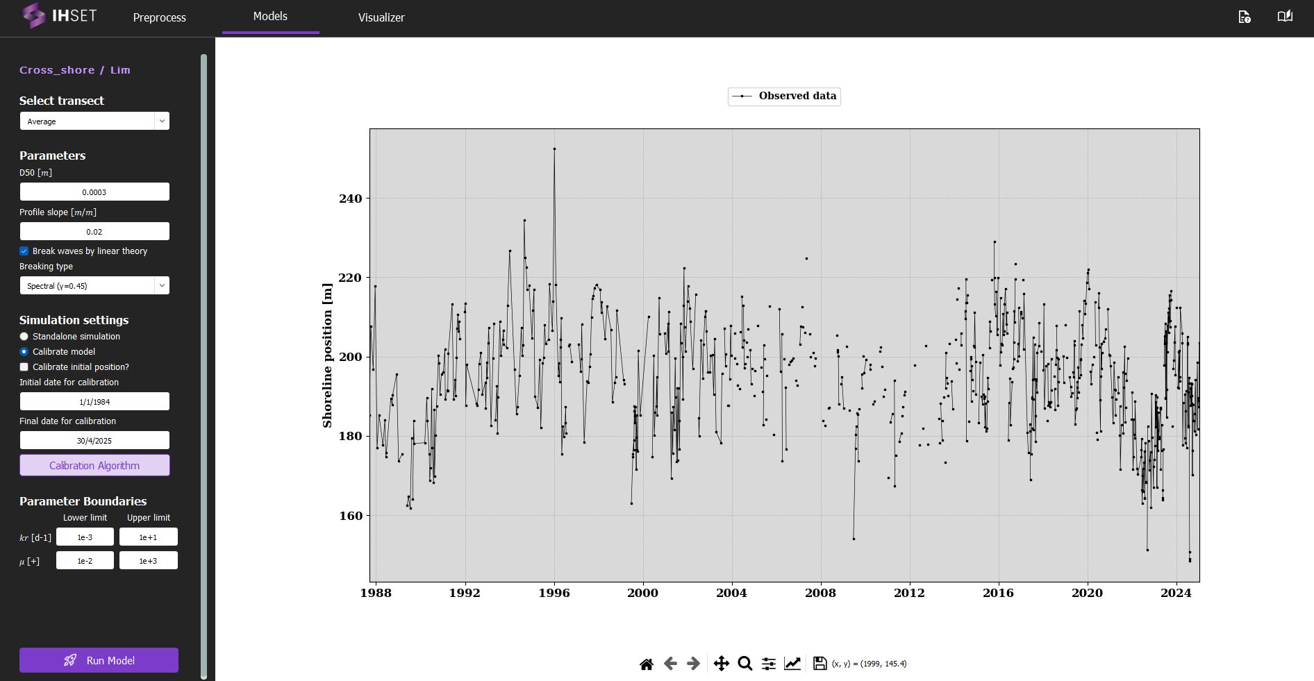
Fig. 3-3-1-6-1. Start screen for simulating the Lim et al. (2022) model.
Simulation inputs
This section outlines the input file, parameters, and simulation settings necessary to run this model in accordance with the procedure provided in the previous section.
NetCDF file
The primary input to run the Lim et al. (2022) model is the NetCDF file produced using the Preprocess module. More information about the contents of this dataset can be found here. This file provides the wave forcing data, comprised of wave data and optionally sea level data, which is inputted directly into the equations for the model. The NetCDF also contains the shoreline observation data, which is used to calibrate the model. For more information about the calibration process and parameters, please check the Calibration section.
As mentioned in the Simulation Procedure, this file is inputted in the Module tab prior to selecting the model. Once the required data for simulation is added and the model is selected, the screen transitions to the view shown in Fig. 3-3-1-6-1 above.
Parameters
In addition to the NetCDF file provided, a number of parameters must be entered into the module on the left side of the interface. These parameters are assumed to be constant over time and are included as constants in this model as follows:
D50 \([m]\) : Median grain size (Range : [0 ~ 2.0e-3])
Profile slope : Beach profile slope (Range : [0 ~ 0.1])
If “Break waves by linear theory” is selected, the user will have the option to select the Breaking type (spectral or monochromatic), which determines the breaker index (\(γ\)) used.
Calibration Settings
Finally, the simulation settings and parameter boundaries must be selected for calibration. In the side panel, the user can decide to run a standalone simulation or to calibrate the model, described as follows:
Standalone simulation: The model is run with no calibration required, as the date range and parameter values will be entered manually. The option to use the first observation as the initial shoreline position (\(Y_0\)) or to enter it manually will also be given.
Calibrate model: As opposed to the standalone simulation, this will run the model with calibration. The user can then decide whether or not to calibrate the initial position, \(Y_0\).
When calibrating the model, the default initial and final dates for calibration will coincide with the start of the wave data and the end of the shoreline data respectively, though these values can be modified to better suit the data used and the desired output. The user also has the option to modify the calibration algorithm and the parameter boundaries. Though it is not necessary to modify these elements, doing so may can improve the performance or run time of the model.
Simulation results
Using the dataset provided along with the IH-SET software for Angourie Back Beach, Australia, running the model simulation yields several detailed outputs as shown in Fig. 3-3-1-6-2:
Comparison of Model Simulation Results and Observed Data: This shows the differences between the model’s shoreline position predictions and actual observed data over the simulation period.
Time-Series Variation of Forcing Variables: Displays changes in key forcing variables, such as wave climate and sediment transport, over time, providing context for the shoreline response.
Parameter Table Using Calibration Algorithm: Lists the parameters optimized for the model simulation, which are derived from calibration processes to enhance model accuracy.
Calibration and Validation Metrics: A table summarizing performance indicators such as RMSE (Root Mean Square Error), NS (Nash-Sutcliffe Efficiency), R² (Coefficient of Determination), and Bias, assessing the model’s predictive accuracy during both calibration and validation phases.
These outputs together provide a comprehensive view of model performance and reliability, allowing users to evaluate and interpret the shoreline evolution predicted by the simulation.
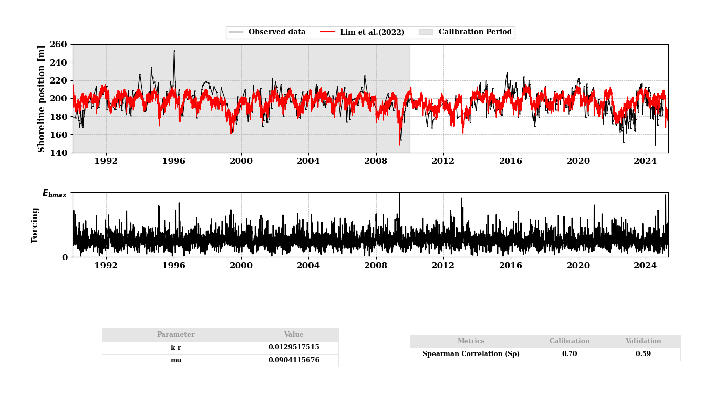
Fig. 3-3-1-6-2. Simulation results for Lim et al. (2022).
In addition, several other functionalities enhance the usability of the model simulation interface:
“Save Results” Button: Allows users to save the simulation results to an output NetCDF file, enabling further analysis or documentation of the model output. All saved simulations can be viewed in the “Visualizer” to compare the results with other EBSEM models, facilitating a side-by-side evaluation of model performance. For more details, please check Visualizer
Other buttons: These buttons allow users to customize and adjust the figures related to the simulation results. Users can modify visual elements such as axis labels, graph types, or legends for clearer interpretation or presentation. Once the desired adjustments are made, users can save the figures in various formats for further use or reporting.
These features enable users not only to analyze and retain results but also to compare multiple models effectively for enhanced decision-making in shoreline evolution modeling.