Dean (1991)
Description
Dean (1991) serves as one of the fundamental studies on the characteristics and applications of equilibrium beach profiles in coastal engineering. This study is most well known for its applications of the simple equilibrium beach profile equation based on wave energy dissipation taking the form proposed by Bruun (1954) and supported by Dean (1997) (Fig. 3-2-1-1-1):
\(h\) : the water depth
\(x\) : the seaward distance
\(A\) : the Dean parameter
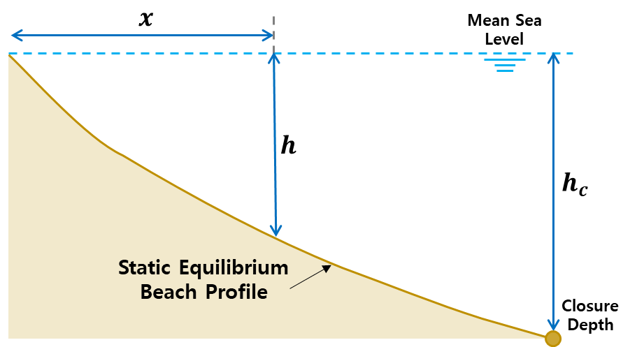
Fig. 3-2-1-1-1. Definition sketch of equilibrium beach profile model (Dean, 1991).
The Dean parameter included in this equation is a scale parameter depending on wave climate and sediment characteristics, and has been defined using linear wave theory as follows:
\(𝒟\) : the energy dissipation per unit volume
\(D\) : the sediment particle diameter
\(ρ\) : the water mass density
\(g\) : gravity
\(κ\) : the constant relating wave height to water depth within surf zone
This study demonstrates the utility of the proposed equation using several examples while assuming that the wave height with the surf zone is proportional to the local water depth within the proportionality parameter, κ = 0.78. Dean (1991) then goes on to define the three profile types that can develop relative to sediment grain size, as well as the five equilibrium profile types that may develop relative to an initial uniform slope that is out of equilibrium. These findings are intended to serve as a framework to predict coastal project performance and the behavior of natural beach systems.
Simulation procedure
The following describes the procedure for simulating the Dean (1991) model. The figure below illustrates the start screen for simulating the model.
Upload the required file (see NetCDF file in Simulation inputs below) using the Browse File button in the Models tab.
Select the desired model from the list of modules to open the model’s start screen.
Adjust the input parameters in the side panel according to the model’s requirements (Please see Parameters & Calibration in Simulation settings)
Optionally, provide bathymetry data by clicking the “Open CSV (Beach Profile)” button and navigating to the desired CSV containing the beach profile, as described below.
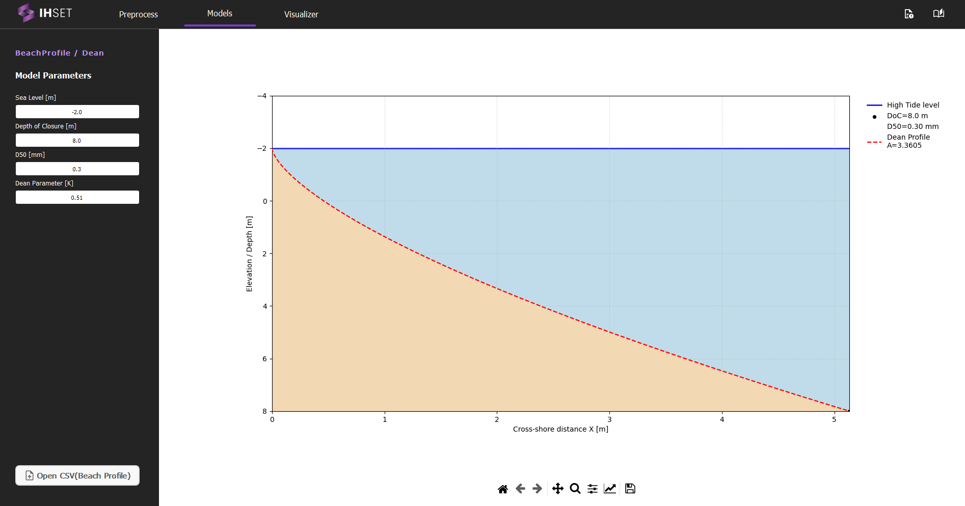
Fig. 3-1-1-1-2. Start screen for simulating the Dean (1991) model.
Simulation settings
Parameters
To run this model, the following parameters are necessary:
Seal Level : Mean sea level (MSL) \([m]\). This is relative to the depth, so a negative number indicates a MSL above 0.
Depth of closure : Depth of closure \([m]\)
D50 : Median grain size \([mm]\)
Dean Parameter \([A]\) : The resulting Dean Parameter calculated using the other three parameters. This parameter can also be entered independent of the values provided.
Bathymetry Dataset (CSV)
The user has the option to upload a reference beach profile in the form of a CSV file containing the following columns:
x : the offshore distance from shoreline \([m]\)
z : the water depth according to the offshore distance \([m]\)
By clicking the “Open CSV (Beach Profile)” button (see Fig. 3-1-1-1-2), the user can load the CSV file containing the dataset for plotting and calibration. It is important to note that the calibration completed by this model is not as intensive as seen in other models and in the Calibration section, as explained further below.
Calibration of the Dean profile with field data.
Once the user provides the optional bathymetry data, the model will automatically calibrate, generating a new Dean Parameter that is fit to the loaded profile using the parameters provided. If the user modifies any of the parameters, the model can be recalibrated using the “Calibrate Equilibrium Profile” button.
For the calibration of the Dean model, a beach profile measured in the field with X,Y input data can be used, where X is the distance of the profile perpendicular to the coastline and Z is the vertical variation of the profile from the zero reference point.
The example below shows the input CSV file format for the Dean model for calibration with field profile data, where it is important to highlight the presence of the X,Y header for the correct loading of data when using the button: “Open CSV (Beach Profile)”:
X,Y
0.0,-5.8508468
1.0137528294529534,-5.80088
2.027505658905907,-5.7509133
3.04125848835886,-5.7009465
4.055011317811814,-5.6521598
5.068764147264767,-5.602193
6.08251697671772,-5.5522262
7.096269806170674,-5.5022595
8.110022635623627,-5.4522927
9.12377546507658,-5.4023259
10.137528294529535,-5.3535392
...
452.1337619360172,12.995833
453.1475147654702,13.101818
454.1612675949231,13.231795
Note: The high tide level (HTL) and depth of closure (DoC), can be adjusted in the model parameters, and a new recalibration of the loaded profile may be requested.
Example dataset for calibration (Download)
An example beach profile dataset compatible with the Dean (1991) calibration workflow is available for download below.
Download example ZIP:
sha256:e56b5fd740e8c5bd44487d4a407392f676139e34571c9f6be054c98bae1c42aa
Calibration is performed using the least squares method by approximation along the X-axis (Figure 3-1-1-1-3).
The model simulation generates a graph of the beach equilibrium profile using Dean’s (1991) formulation. The side menu buttons on the screen shown in Figure 3-1-1-1-3 allow users to customize and adjust the figures related to the simulation results. Users can modify visual elements, such as axis labels, graph types, or legends, for clearer interpretation or presentation. After making the desired adjustments, users can save the figures in various formats for later use or report preparation.
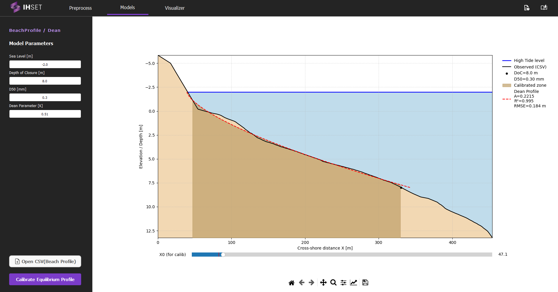
Fig. 3-1-1-1-3. Simulation results according to the settings for Dean (1991).