Jaramillo et al. (2021a)
Description
Jaramillo et al. (2021a) proposed a model based on the kinetic equation defined by Yates et al. (2009). The proposed model also adapts the methodology of Turki et al. (2013), considering that beach rotation is independent of other movements and dependent on incident wave conditions. Regarding incident wave conditions, the study assumes waves along the beach are homogeneous and uniform across the shoreline. Thus, Jaramillo et al. (2021a) suggested a shoreline rotation model that predicts the temporal evolution of the shoreline orientation based on the concept of previous research and the observation data as follows (Fig. 3-3-2-2-1):
\(P\) : the incoming wave power related to the significant wave height \(H_s\) and the wave peak period \(T_p\) as \(P=H_s^2T_p\)
\(α_{s,eq}\) : the asymptotical equilibrium shoreline orientation
\(α_s(t)\) : the shoreline orientation at time \(t\)
\(L^±\) : the proportional constants where \(L^+\) indicates the clockwise shoreline rotation and \(L^-\) indicates the counterclockwise rotation, respectively
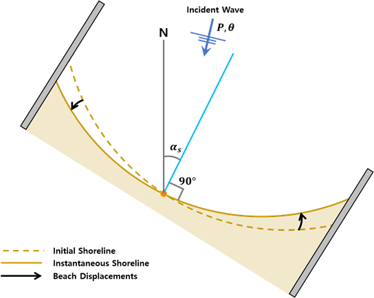
Fig. 3-3-2-2-1. Definition sketch of shoreline rotation model proposed by Jaramillo et al. (2021a).
Here, the shoreline orientation is defined as the angle between the line perpendicular to the linear-regression fit and geographic north (Fig. 3-3-2-2-2). Jaramillo et al. (2021a) suggested the linear relationship between the asymptotical equilibrium of shoreline orientation and the incident wave direction as follows:
\(θ\) : the incident wave direction
\(a',b'\) : the empirical parameters that satisfy the linear relationship
The model proposed by Jaramillo et al. (2021a) is suited for application at microtidal beaches with similar sediment grain sizes and intermediate beach states. Similar to Turki et al. (2013), though, this model is subject to several assumptions that may limit its application across differing beaches. Additionally, since some of the model parameters remain constant during execution, the model cannot accurately reproduce variability resulting from changes in storm intensity, the rate of sea-level rise, or human interventions.
Simulation procedure
The following describes the procedure for simulating the Jaramillo et al. (2021a) model. The figure below illustrates the start screen for simulating the model.
Upload the required file (see NetCDF file in Simulation inputs below) using the Browse File button in the Models tab.
Select the desired model from the list of modules to open the model’s start screen.
Adjust the input parameters and simulation settings in the side panel according to the model’s requirements (see Calibration settings in Simulation inputs below).
Click on the “Run Model” button to start the model execution.
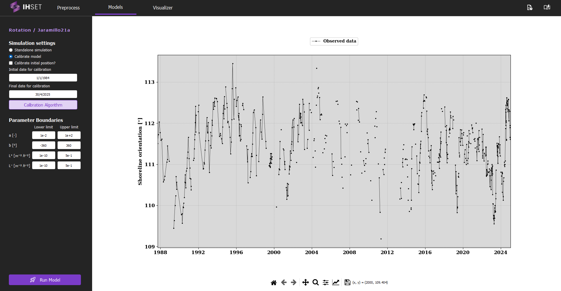
Fig. 3-3-2-2-3. Start screen for simulating the Jaramillo et al. (2021a) model.
Simulation inputs
This section outlines the input file, parameters, and simulation settings necessary to run this model in accordance with the procedure provided in the previous section.
NetCDF file
The primary input to run the Jaramillo et al. (2021a) model is the NetCDF file produced using the Preprocess module. More information about the contents of this dataset can be found here. This file provides the wave forcing data, comprised of wave data and optionally sea level data, which is inputted directly into the equations for the model. The NetCDF also contains the shoreline observation data, which is used to calibrate the model. For more information about the calibration process and parameters, please check the Calibration section.
As mentioned in the Simulation Procedure, this file is inputted in the Module tab prior to selecting the model. Once the required data for simulation is added and the model is selected, the screen transitions to the view shown in Fig. 3-4-2-2 above.
Calibration Settings
No additional parameters must be entered for this model, so the only other inputs are the simulation settings and parameter boundaries for calibration. In the side panel, the user can decide to run a standalone simulation or to calibrate the model, described as follows:
Standalone simulation: The model is run with no calibration required, as the date range and parameter values will be entered manually. The option to use the first observation as the initial shoreline position (\(a_0\)) or to enter it manually will also be given.
Calibrate model: As opposed to the standalone simulation, this will run the model with calibration. The user can then decide whether or not to calibrate the initial position, \(α_0\).
When calibrating the model, the default initial and final dates for calibration will coincide with the start of the wave data and the end of the shoreline data respectively, though these values can be modified to better suit the data used and the desired output. The user also has the option to modify the calibration algorithm and the parameter boundaries. Though it is not necessary to modify these elements, doing so may can improve the performance or run time of the model.
Assimilation by Ensemble Kalman Filter (EnKF): The Ensemble Kalman Filter (EnKF) is a sequential data assimilation technique used to optimally combine model predictions and observations for dynamic, potentially non-linear systems. The EnKF represents the system state using an ensemble of realizations, allowing the estimation of statistical moments (mean and covariance) directly from the ensemble. Each realization is propagated forward using the model dynamics, and updated whenever observations become available.
The method consists of two main steps:
Forecast step:
Each ensemble member is propagated forward using the model:\[ \mathbf{x}_t^{(k)} = \Phi\left(\mathbf{x}_{t-1}^{(k)}\right) \]where \(\mathbf{x}_t^{(k)}\) is the state vector of ensemble member \(k\), and \(\Phi\) represents the (possibly non-linear) model operator.
Update step:
The ensemble is updated using observations \(\mathbf{y}_t\):\[ \mathbf{x}_t^{(k)} \leftarrow \mathbf{x}_t^{(k)} + \mathbf{K} \left( \mathbf{y}_t + \boldsymbol{\epsilon}_t^{(k)} - \mathbf{H}\mathbf{x}_t^{(k)} \right) \]where:
\(\mathbf{H}\) is the observation operator,
\(\boldsymbol{\epsilon}_t^{(k)}\) represents observation noise,
\(\mathbf{K}\) is the Kalman gain matrix.
The Kalman gain controls the balance between model predictions and observations and is defined as:
where:
\(\mathbf{C}_{xx}\) is the forecast state covariance estimated from the ensemble,
\(\mathbf{R}\) is the observation error covariance matrix.
Key characteristics:
Approximates mean and covariance using an ensemble of realizations.
Suitable for non-linear and high-dimensional systems.
Sequentially assimilates data as observations become available.
Can update both:
Model state variables
Model parameters (augmented state formulation)
Naturally incorporates uncertainty from both model and observations.
Application in IH-SET:
When enabled, the EnKF allows the model to assimilate observational data during simulations, dynamically correcting shoreline predictions and improving parameter estimation. This is particularly beneficial for systems with strong temporal variability and limited observational coverage.
Simulation results
Using the dataset provided along with the IH-SET software for Angourie Back Beach, Australia, running the model simulation yields several detailed outputs as shown in Fig. 3-3-2-2-5:
Comparison of Model Simulation Results and Observed Data: This shows the differences between the model’s orientation predictions and actual observed data over the simulation period.
Time-Series Variation of Forcing Variables: Displays changes in key forcing variables, such as wave climate and sediment transport, over time, providing context for the orientation response.
Parameter Table Using Calibration Algorithm: Lists the parameters optimized for the model simulation, which are derived from calibration processes to enhance model accuracy.
Calibration and Validation Metrics: A table summarizing performance indicators such as RMSE (Root Mean Square Error), NS (Nash-Sutcliffe Efficiency), R² (Coefficient of Determination), and Bias, assessing the model’s predictive accuracy during both calibration and validation phases.
These outputs together provide a comprehensive view of model performance and reliability, allowing users to evaluate and interpret the shoreline evolution predicted by the simulation.
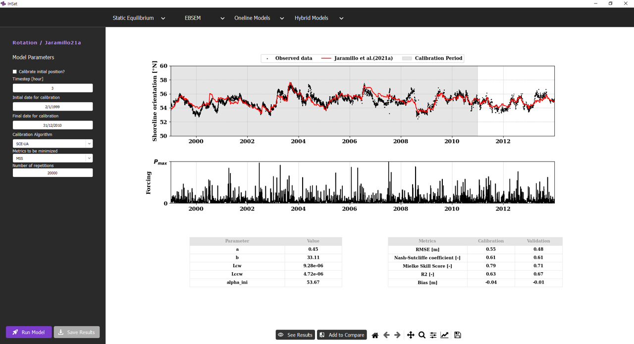
Fig. 3-3-2-2-5. Simulation results for Jaramillo et al. (2021a).
In addition, several other functionalities enhance the usability of the model simulation interface:
“Save Results” Button: Allows users to save the simulation results to an output NetCDF file, enabling further analysis or documentation of the model output. All saved simulations can be viewed in the “Visualizer” to compare the results with other EBSEM models, facilitating a side-by-side evaluation of model performance. For more details, please check Visualizer
Other buttons: These buttons allow users to customize and adjust the figures related to the simulation results. Users can modify visual elements such as axis labels, graph types, or legends for clearer interpretation or presentation. Once the desired adjustments are made, users can save the figures in various formats for further use or reporting.
These features enable users not only to analyze and retain results but also to compare multiple models effectively for enhanced decision-making in shoreline evolution modeling.