Hsu and Evans (1989)
Description
Hsu and Evans (1989) proposed the Parabolic Bay Shape Equation (PBSE), a beach planform model applicable to crenulate-shaped bays formed between two headlands. In these environments, the incident waves approach the bay from a predominant direction and arrive at a diffraction point before proceeding toward the beach with some refraction. For a bay in static equilibrium, the waves then break simultaneously along the beach. Unlike the logarithmic spiral equation proposed earlier by Silvester (1960), this equation assumes the beach will thus follow a parabolic shape to better capture the downcast region of the bay as follows (Fig. 3-2-2-1-1):
\(R\) : the radius measured from the tip of the headland breakwater
\(R_o\) : the length of the control line joining the updrift diffraction point to the down-coast control point
\(θ\) : the angle between the location of \(R\) on the shoreline
\(β\) : the angle between the control line and the wavefront at the diffraction point
\(C_i\) : the calibration parameters that depend on the wave obliquity (\(β\)) based on measured shapes of the model beaches (\(i\)=0,1 and 2)
González and Medina (2001) examined the applicability of this equation, determining that the procedure proposed by Hsu and Evans (1989) functioned well for fully developed beaches but required additional criteria to test the stability of undeveloped beaches or predict new undeveloped beaches. For this reason, González and Medina (2001) proposed the methodology for estimating the location of the down-coast limit distance R_o from the control point as a function of \(α_{min}(=90°-β)\) (Fig. 3-2-2-1-1):
\(Y\) : the distance from the control point to the straight alignment down-coast
\(L_s\) : the scaling wavelength calculated by the peak wave period and the wave depth at the diffraction point
\(β_r\) : the angular parameter with a calculated value of 2.13 obtained by comparing 26 Spanish beaches
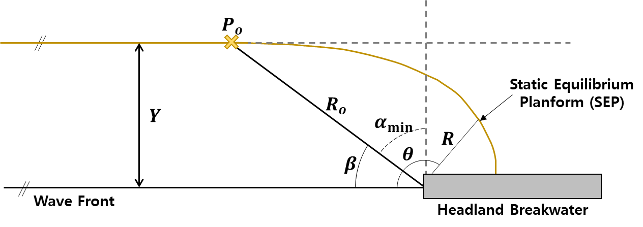
Fig. 3-2-2-1-1. Definition sketch of the static equilibrium planform proposed by Hsu and Evans (1989).
Additionally, González and Medina (2001) demonstrates a methodology to test the stability of a crenulate beach or design a new one in static equilibrium, as well as an analysis of salient formation behind a breakwater, which can be applied using IH-SET.
Simulation settings
Parameters
Wave Fronts : Angle relative to north where the wave crest line and wave diffraction pointer meet
Ts : Significnat wave period to calculate \(L_s\) \([s]\) (Range : [0 ~ 20.0])
Depth Control : Water depth at the diffraction point to calculate \(L_s\) \([m]\) (Range : [0 ~ 20.0])
Lr : Extended planform length from the coastal point \([m]\) (Range : [0 ~ 3000])
Control Point [lat, lon] : Control Point to calculate the static equilibrium planform
Simulation procedure
The following describes the procedure for simulating the static equilibrium planform model. The figure below illustrates the start screen for simulating the model.
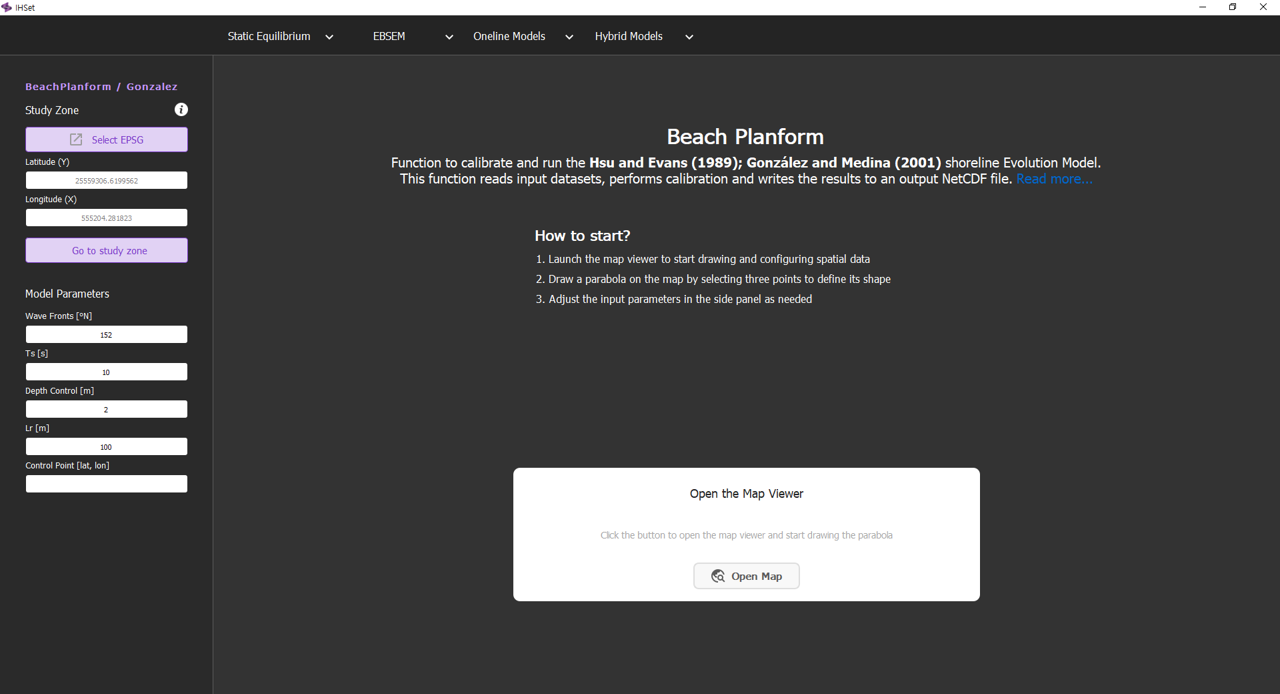
Fig. 3-2-2-1-2. Start screen for simulating the static equilibrium planform model.
Check Coordinate Systems: Coordinate System Alignment is essential to overlay the map image and equilibrium planform data correctly. If the map image and the data use different coordinate systems (e.g., UTM, WGS84), one must transform either the data or the map to match the same coordinate system. Selecting the desired coordinate system, as shown in Fig. 3-2-2-1-3, allows the software to perform this function.
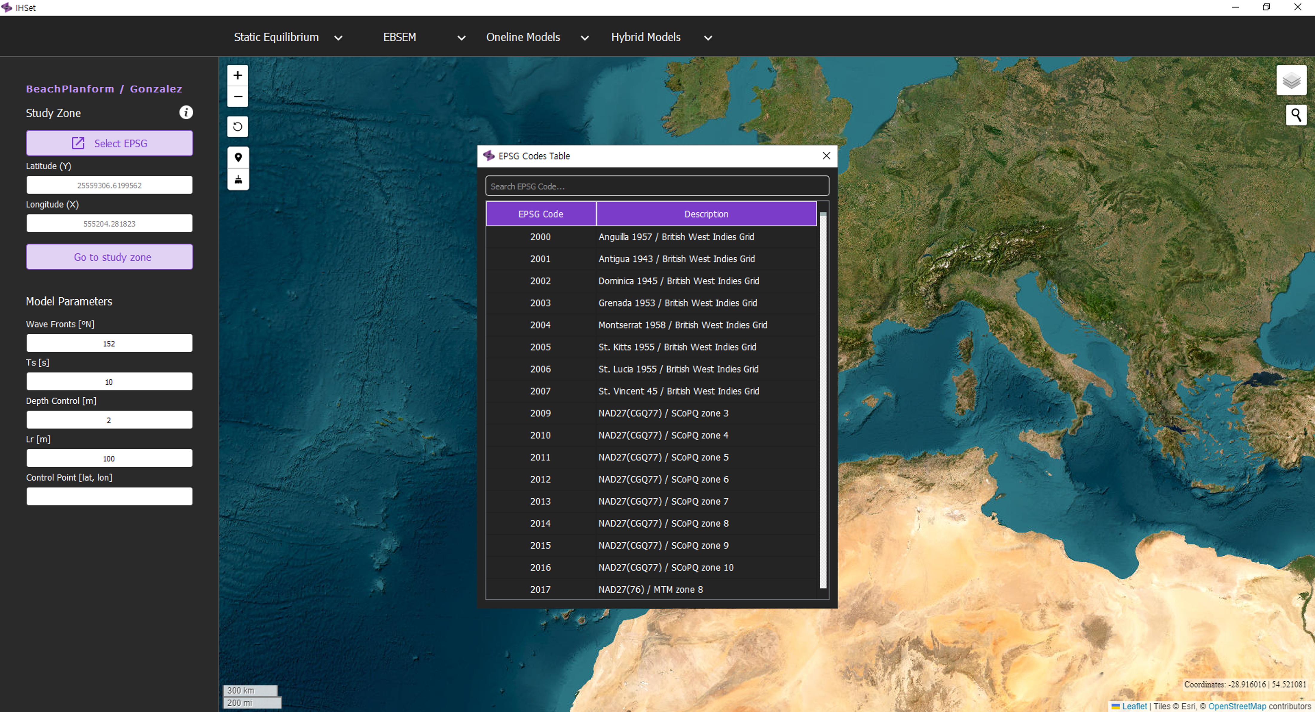
Fig. 3-2-2-1-3. Coordinate system alignment according to the settings for Hsu and Evans (1989).
Navigate to the desired study site: To navigate to the desired study site, enter the coordinates and click the “Go to Study Zone” button, or click the “Find Study Site” button and type the location name.
Plot the static equilibrium planform: Enter the model parameters, click the Point-Click Button, and select the three points on the map to plot the parabola of the static equilibrium shoreline. In order of selection, these points should be the diffraction (control) point, the point of the beach closest to the diffraction point, and the point of the beach furthest from the diffraction point.
Adjust the static equilibrium planform: Adjust the input parameters in the side panel and the selected points on the map as needed. Click the Rotation button and use the red arrow that appears on the map to rotate the predicted planform.
Simulation results
Through this procedure, running the model simulation produces the results shown in Fig. 3-2-2-1-4. These outputs together provide a comprehensive view of model performance and reliability, allowing users to evaluate and interpret the static equilibrium planform predicted by the simulation.
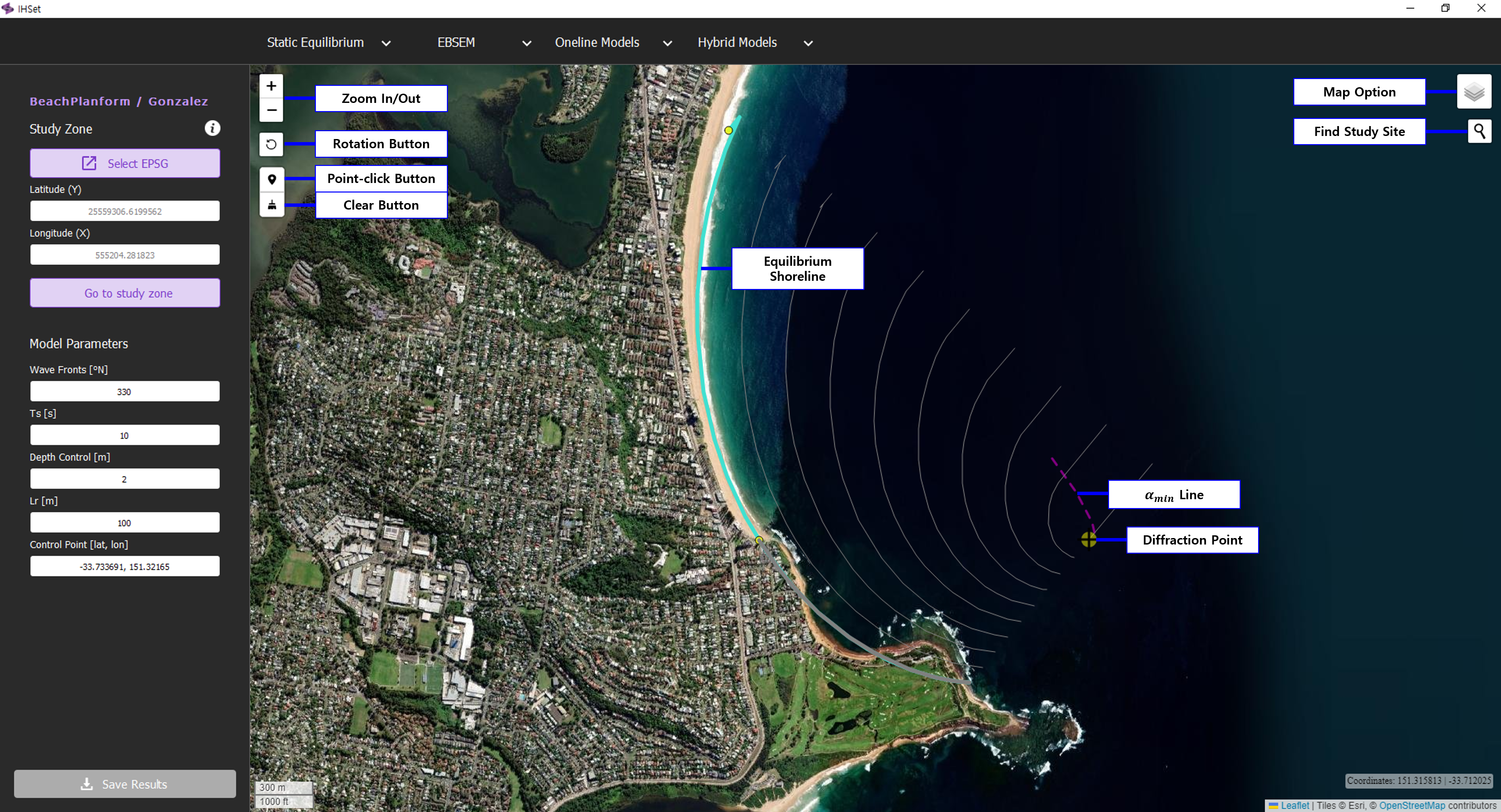
Fig. 3-2-2-1-4. Simulation results according to the settings for Hsu and Evans (1989).
In addition, several other functionalities enhance the usability of the model simulation interface as shown in Fig. 3-2-2-1-4:
“Map Option” Button: Click the Map Option Button to change the display options of the map, such as switching between OpenStreetMap, Google Earth, ESRI World Imagery, and other map layers.
“Zoom In/Out” Button: The Zoom In/Out Buttons allow you to adjust the view of the map by magnifying or reducing the visible area. Alternatively, you can adjust the zoom level using the mouse scroll wheel.
“Clear” Button: The Clear Button is used to reset or remove any drawn elements, markers, or selections on the map, allowing you to start with a clean slate.
“Save Results” Button: Allows users to save the simulation results as a CSV file, enabling further analysis or documentation of the model output.