Jaramillo et al. (2020)
Description
Jaramillo et al. (2020) suggested a shoreline evolution model based on the kinetic equation proposed by Yates et al. (2009). The governing equation of the kinetic equation is defined as follows:
\(S(t)\) : the shoreline position at time \(t\)
\(S_{eq}\) : the equilibrium shoreline position
\(C^±\) : the free parameters where \(C^+\) indicates the accretion and \(C^-\) indicates the erosion, respectively
\(E\) : the incoming breaking wave energy related to the breaking wave height (water depth at breaking \(h_b\) and breaking index γ) as
\(E_{eq}\) : the equilibrium wave energy corresponding to the current shoreline position
Jaramillo et al. (2020) aimed to expand the application of the Yates et al. (2009) model to study cases experiencing noted trends of sediment gains or losses in the medium to long term. As done by several authors prior, this proposed model incorporated a constant linear trend term to account for unexplained shoreline motions uncorrelated with short-term wave climate changes. This constant is introduced within the Equilibrium Energy Function (EEF) and represents the trend rate of sediment gain or loss, related to unresolved processes and multiple natural and anthropic origins. Ultimately, Jaramillo et al. (2020) derived the equilibrium shoreline position by considering the linear trend of the shoreline position as presented in the EEF below:
\(a,b\) : the parameters that satisfy the energy equilibrium function
\(v_{lt}\) : the linear trend term according to the sediment gain/loss on the littoral zone
Fig. 3-3-1-5-1 shows that model predictions with a linear trend term outperform those without the term. The figure shows that the mean shoreline position increases over time due to sand gain/loss.
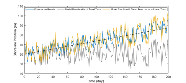
Fig. 3-3-1-5-1. Concept of the shoreline evolution model with the linear trend term proposed by Jaramillo et al. (2020).
With the addition of the linear trend term, the model proposed by Jaramillo et al. (2020) can be applied across a variety of temporal scales. Additionally, it is less complex than previous empirical evolution models and requires fewer calibration parameters to be more computationally efficient.
Simulation procedure
The following describes the procedure for simulating the Jaramillo et al. (2020) model. The figure below illustrates the start screen for simulating the model.
Upload the required file (see NetCDF file in Simulation inputs below) using the Browse File button in the Models tab.
Select the desired model from the list of modules to open the model’s start screen.
Adjust the input parameters and simulation settings in the side panel according to the model’s requirements (see Calibration settings in Simulation inputs below).
Click on the “Run Model” button to start the model execution.
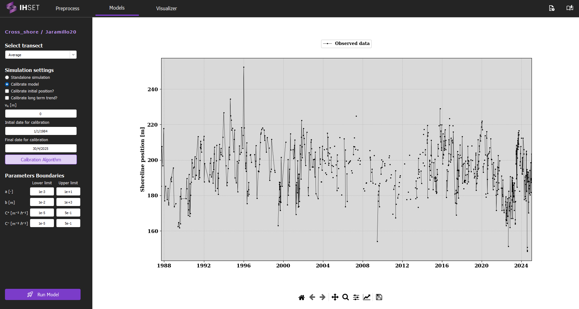
Fig. 3-3-1-5-2. Start screen for simulating the Jaramillo et al. (2020) model.
Simulation inputs
This section outlines the input file, parameters, and simulation settings necessary to run this model in accordance with the procedure provided in the previous section.
NetCDF file
The primary input to run the Jaramillo et al. (2020) model is the NetCDF file produced using the Preprocess module. More information about the contents of this dataset can be found here. This file provides the wave forcing data, comprised of wave data and optionally sea level data, which is inputted directly into the equations for the model. The NetCDF also contains the shoreline observation data, which is used to calibrate the model. For more information about the calibration process and parameters, please check the Calibration section.
As mentioned in the Simulation Procedure, this file is inputted in the Module tab prior to selecting the model. Once the required data for simulation is added and the model is selected, the screen transitions to the view shown in Fig. 3-3-1-5-2 above.
Calibration Settings
No additional parameters must be entered for this model, so the only other inputs are the simulation settings and parameter boundaries for calibration. In the side panel, the user can decide to run a standalone simulation or to calibrate the model, described as follows:
Standalone simulation: The model is run with no calibration required, as the date range and parameter values will be entered manually. The option to use the first observation as the initial shoreline position (\(Y_0\)) or to enter it manually will also be given.
Calibrate model: As opposed to the standalone simulation, this will run the model with calibration. The user can then decide whether or not to calibrate the initial position, \(Y_0\), and the long term trend, \(v_{lt}\). The \(v_{lt}\) must be entered manually if it is not calibrated.
When calibrating the model, the default initial and final dates for calibration will coincide with the start of the wave data and the end of the shoreline data respectively, though these values can be modified to better suit the data used and the desired output. The user also has the option to modify the calibration algorithm and the parameter boundaries. Though it is not necessary to modify these elements, doing so may can improve the performance or run time of the model.
Assimilation by Ensemble Kalman Filter (EnKF): The Ensemble Kalman Filter (EnKF) is a sequential data assimilation technique used to optimally combine model predictions and observations for dynamic, potentially non-linear systems. The EnKF represents the system state using an ensemble of realizations, allowing the estimation of statistical moments (mean and covariance) directly from the ensemble. Each realization is propagated forward using the model dynamics, and updated whenever observations become available.
The method consists of two main steps:
Forecast step:
Each ensemble member is propagated forward using the model:\[ \mathbf{x}_t^{(k)} = \Phi\left(\mathbf{x}_{t-1}^{(k)}\right) \]where \(\mathbf{x}_t^{(k)}\) is the state vector of ensemble member \(k\), and \(\Phi\) represents the (possibly non-linear) model operator.
Update step:
The ensemble is updated using observations \(\mathbf{y}_t\):\[ \mathbf{x}_t^{(k)} \leftarrow \mathbf{x}_t^{(k)} + \mathbf{K} \left( \mathbf{y}_t + \boldsymbol{\epsilon}_t^{(k)} - \mathbf{H}\mathbf{x}_t^{(k)} \right) \]where:
\(\mathbf{H}\) is the observation operator,
\(\boldsymbol{\epsilon}_t^{(k)}\) represents observation noise,
\(\mathbf{K}\) is the Kalman gain matrix.
The Kalman gain controls the balance between model predictions and observations and is defined as:
where:
\(\mathbf{C}_{xx}\) is the forecast state covariance estimated from the ensemble,
\(\mathbf{R}\) is the observation error covariance matrix.
Key characteristics:
Approximates mean and covariance using an ensemble of realizations.
Suitable for non-linear and high-dimensional systems.
Sequentially assimilates data as observations become available.
Can update both:
Model state variables
Model parameters (augmented state formulation)
Naturally incorporates uncertainty from both model and observations.
Application in IH-SET:
When enabled, the EnKF allows the model to assimilate observational data during simulations, dynamically correcting shoreline predictions and improving parameter estimation. This is particularly beneficial for systems with strong temporal variability and limited observational coverage.
Simulation results
Using the dataset provided along with the IH-SET software for Angourie Back Beach, Australia, running the model simulation yields several detailed outputs as shown in Fig. 3-3-1-5-3:
Comparison of Model Simulation Results and Observed Data: This shows the differences between the model’s shoreline position predictions and actual observed data over the simulation period.
Time-Series Variation of Forcing Variables: Displays changes in key forcing variables, such as wave climate and sediment transport, over time, providing context for the shoreline response.
Parameter Table Using Calibration Algorithm: Lists the parameters optimized for the model simulation, which are derived from calibration processes to enhance model accuracy.
Calibration and Validation Metrics: A table summarizing performance indicators such as RMSE (Root Mean Square Error), NS (Nash-Sutcliffe Efficiency), R² (Coefficient of Determination), and Bias, assessing the model’s predictive accuracy during both calibration and validation phases.
These outputs together provide a comprehensive view of model performance and reliability, allowing users to evaluate and interpret the shoreline evolution predicted by the simulation.
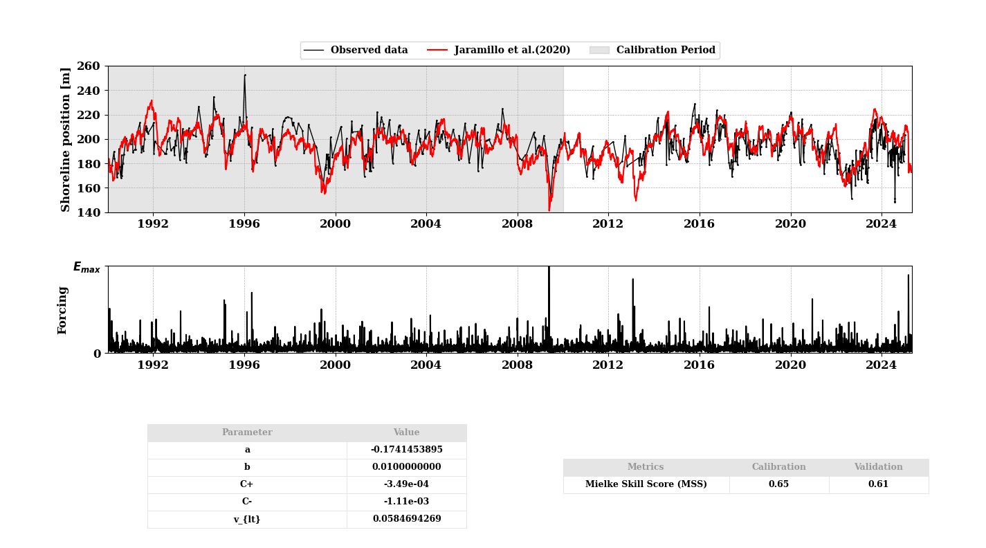
Fig. 3-3-1-5-4. Simulation results for Jaramillo et al. (2020).
In addition, several other functionalities enhance the usability of the model simulation interface:
“Save Results” Button: Allows users to save the simulation results to an output NetCDF file, enabling further analysis or documentation of the model output. All saved simulations can be viewed in the “Visualizer” to compare the results with other EBSEM models, facilitating a side-by-side evaluation of model performance. For more details, please check Visualizer
Other buttons: These buttons allow users to customize and adjust the figures related to the simulation results. Users can modify visual elements such as axis labels, graph types, or legends for clearer interpretation or presentation. Once the desired adjustments are made, users can save the figures in various formats for further use or reporting.
These features enable users not only to analyze and retain results but also to compare multiple models effectively for enhanced decision-making in shoreline evolution modeling.