3.1. Preprocess

Data preprocessing to perform simulations in IH-SET involves several stages. In the first stage, the user must provide input files in CSV or IH-Data format, containing the key variables to feed the IH-SET models (minimum information that the models require): (1) significant wave height (Hs), (2) peak period (Tp), (3) wave direction (Dir), (4) observation data on the position and/or orientation of the coastline; all data must have (5) spatial reference (geographic coordinates) and (6) associated date/time information. Additionally, data on (7) mean sea level changes, (8) including tidal fluctuation and (9) storm surge can be incorporated to refine the simulations. In the second stage, the data are converted to the NetCDF file format, which is more suitable for storing multidimensional scientific data. Figure 3.1. Shows the infographic of the preprocess module ilustrating several possibilities of input data to generate the proper NetCDF input file to be processed by the models.

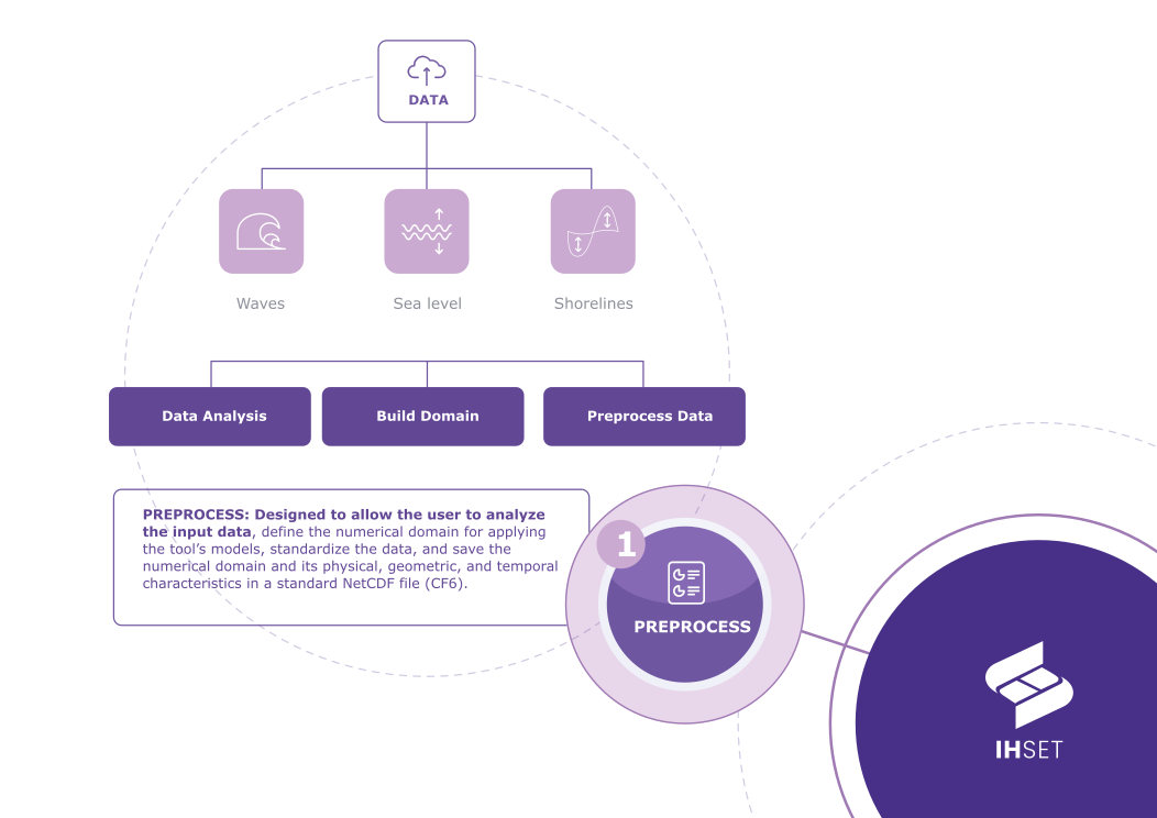Fig. 3_1 Fig. 3-1. The Infographic of the IH-SET Preprocess module.

Proper data preprocessing is essential for the good performance of simulations of coastal evolution processes with the EBSEM, One-line and Hybrid models from the IH-SET application suite. For detailed guidance on preprocessing steps and data formats, see the following sections.

3.1.1. Numerical Domain

Not only does the Preprocess module reformat data, but this tool also establishes the numerical domain that is the foundation for the EBSEM, One-line and Hybrid models. The datum for this domain is a singular baseline drawn parallel to the shoreline observations on their landward side. From this baseline, transects extend perpendicularly and intersect with the shoreline observations. These transects act as distinct, one-dimensional domains originating at the baseline over which shoreline observations are quantified based on the distance of their intersection point from the transect’s origin (Figure 3.1.1.1).

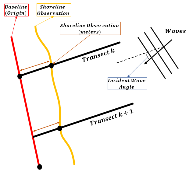Fig. 3_1_1_1_1 Fig. 3-1-1-1. A simplified representation of the numerical domain.

Across the whole domain, it is assumed that the bathymetry close to the shoreline is straight and parallel to the baseline, and thus the shoreline. This is an important assumption, as it allows for the calculation of the bathymetry angle and the significant wave height at breaking (\(H_{s_b}\)), which is the wave forcing input for several models, such as Miller and Dean (2004) and Jara et al. (2015). To calculate \(H_{s_b}\), Snell’s Law is first applied to calculate wave refraction based on the incident wave angle relative to the normal of the shore, which is indicated by the transects. If the transects are not generated perpendicularly to the shoreline, the wave will not be propagated correctly in the calculation of \(H_{s_b}\).

A correctly established numerical domain is also necessary for interpolating wave-forcing data. When multiple files for wave forcing are provided, wave data is interpolated to the endpoint of the nearest transect and assigned to the shoreline observation along that transect. If transects are perpendicular, the shoreline observations will be matched with the closest wave data point. However, if transects cross or are not perpendicular, the wave data and shoreline observations will not be matched correctly (Figure 3.1.1.2).

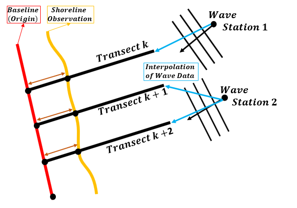Fig. 3_1_1_1_2 Fig. 3-1-1-1-2. A simplified representation of the interpolation of wave data.

Within IH-SET, Cross-shore models are applied across one transect at a time, while the Rotation, One-line, and Hybrid models are applied across the entire numerical domain.

3.1.2. Input dataset

The input dataset for the Preprocess module must include data for wave forcing and shoreline observations to generate the preprocessed dataset. Tide and surge data can also be provided to generate an output dataset that takes into account additional forcings from local sea level variation.

Fig. 3_1_2

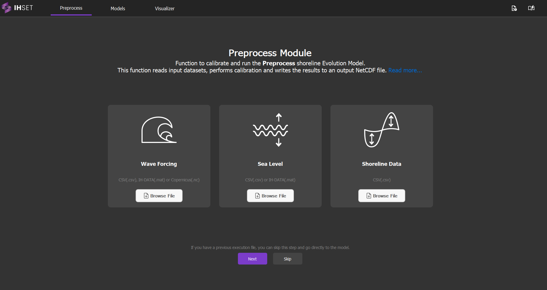
Fig. 3-1-2. Main screen of the Preprocess module with options to load wave, tide, and shoreline data for automatic configuration of the data in the NetCDF input format of the IH-SET.

Note

Input files in CSV format suitable for loading into the Preprocess module, containing wave, tide, and shoreline data, can be downloaded directly from section 4. Test Cases: Download Test Case Files.

3.1.2.1. Input File 1: Wave Forcing (Required)

To accurately model and predict the evolution of the shoreline, it is necessary to input the shoreline location as well as the forcings that changed said location. Thus, it is required that wave forcing data be the first input of the Preprocess module. The user has the option to upload multiple wave forcing datasets of the same format, as the Preprocess module will interpolate the dataset best suited for each transect based on coordinate data.

The input data for wave forcing can be provided in three formats: CSV, NetCDF (Copernicus), or IH-Data. Each time series dataset must include:

Time: Observation date and time in YYYY-MM-DD or YYYY-MM-DDThh:mm:ss.sssZ format.
Hs: Significant wave height in meters (m), representing the average height of the highest one-third of waves. Named VHM0 in NetCDF files.
Tp: Peak period in seconds (s), indicating the time between successive wave crests. Named VTPK in NetCDF files.
Dir: Wave direction, expressed as the angle in degrees from true north. Named VMDR in NetCDF files. If uploading a NetCDF file, the variables for spectral moments (-1,0) and (0,2) wave periods must also be included (VTM10 and VTM02).

IH-SET accepts time series for a single point or for multiple wave points near the surf zone or beach closure profile. For cases involving multiple wave points, it is important to name the input CSV files with the same base name, but numbering the end of the file names according to the order of the associated beach profiles, as in the example below in a beach with 15 beach profiles and 15 wave points:

Suggested name for wave files according to transect association:

nearshore_waves_timeseries_transect_01.csv
nearshore_waves_timeseries_transect_02.csv
nearshore_waves_timeseries_transect_03.csv
…
nearshore_waves_timeseries_transect_15.csv

The data in each CSV should have a header with the variable names as in the example below, using the first 10 lines of one of the input CSVs:

nearshore_waves_timeseries_transect_01.csv content:

time,Hs,Tp,Dir
1940-01-02,0.955587402,7.489383124,116.8650704
1940-01-03,0.986981874,5.479013276,87.80441075
1940-01-04,1.426444472,6.420172485,73.51347322
1940-01-05,1.248591206,6.801605915,70.22703469
1940-01-06,0.705501012,6.950942889,79.88670194
1940-01-07,1.146077182,5.482588834,125.5313966
1940-01-08,1.131035458,5.721648541,127.1965788
1940-01-09,0.840004178,6.829882205,109.2263848
1940-01-10,0.843138868,7.927856374,99.3055916
...

Each time series dataset must be accompanied by station data for the wave monitoring station. Coordinates must be provided in the selected coordinate reference system (CRS) as identified by the European Petroleum Survey Group (EPSG). Station data includes:

Lat: Latitude of the station in the selected CRS.
Lon: Longitude of the station in the selected CRS.
EPSG: ESPG conversion code for the selected CRS. Only required for CSV files, as the other two formats list coordinates in the default coordinate system, the World Geodetic System 1984 (WGS84).
Wave Depth: Water depth at the station (m).

The method for providing station data depends on the file type:

CSV (one station): Enter the data into the pop-up that will appear after selecting the CSV file in the Preprocess module.
CSV (multiple stations): Provide a second CSV file containing the station data in columns, with a row for each station. Make sure the rows are in the same order as the station CSV files when selected in the Preprocess module.
NetCDF: Provide a second NetCDF file containing the variable for bathymetry (deptho).
IH-DATA: Bathymetry data should be included with the timeseries dataset. No additional file is necessary.

The following table summarizes each format:

Format	File Type	Timeseries Variables	Additional Station Data	Potential Source
CSV	.csv	`time`,`Hs`,`Tp`,`Dir`	`Lat`,`Lon`,`EPSG`,`Wave Depth`	European Centre for Medium-Range Weather Forecasts (ECMWF) ERA5 or similar database
NetCDF	.nc	`time`,`latitude`,`longitude`,`VHM0`,`VMDR`,`VTPK`	`time`,`latitude`,`longitude`,`deptho`	Copernicus
Global Ocean Waves (GOW) IH-Data	.mat	`time`,`lat`,`lon`,`bat`,`hs`,`tp`,`dir`	–	IH-Data

Example of CSV (multiple stations):

Coordinate file: nearshore_waves_coords.csv:

lon,lat,depth,epsg
342728.49839001364,6261920.365477566,15,32756
342701.13906130445,6261878.3398511065,15,32756
342660.3934545089,6261831.219421092,15,32756
...
342604.74627520185,6261766.866004263,15,32756

Note: For projects with a single wave point near the beach of interest, the wave point coordinate file is not necessary; the single point information can be entered directly into the auxiliary pop-up window that opens immediately after loading just one CSV wave file.

3.1.2.2. Input File 2: Sea Level (Optional)

While wave data is the only forcing input required to run each model, more refined results can be generated when local variations in sea level are accounted for as additional forcings. For this reason, IH-SET can adjust the forcing input using optional sea level data. The input data for shoreline observations can be provided in two formats: CSV or IH-Data. Each dataset must include:

Time: Observation date and time in YYYY-MM-DD or YYYY-MM-DDThh:mm:ss.sssZ format.
Tide or Surge: Sea level reading in meters of the tide or surge respectively. The user has the option to include data for tide, surge, or both.

The following table summarizes each format:

Format	File Type	Required Variables	Potential Source
CSV for tide	.csv	`time`,`tide`	FES or CODEC
CSV for surge	.csv	`time`,`surge`	CODEC
Global Ocean Tide (GOT) IH-Data	.mat	`time`,`tide`	IH-Data
Global Ocean Surge (GOS) IH-Data	.mat	`time`,`zeta`	IH-Data

The examples below show the formatting of the astronomical tide and storm surge files with their respective headers for the Preprocess module to recognize the tidal input data.

Astronomical tide file: tide_timeseries.csv

time,tide
1950-01-01,0.01031358994119
1950-01-02,-0.0001428425773902
1950-01-03,-0.0081518937384059
1950-01-04,-0.0166269009864276
1950-01-05,-0.0236500053011406
1950-01-06,-0.0268531034303317
1950-01-07,-0.0244905341298127
1950-01-08,-0.0163098156375265
1950-01-09,-0.003733772358122
...

Storm surge file: stormSurge_timeseries.csv

time,surge
1979-01-01 00:00:00,0.129
1979-01-01 01:00:00,0.594
1979-01-01 02:00:00,0.96
1979-01-01 03:00:00,1.16
1979-01-01 04:00:00,1.136
1979-01-01 05:00:00,0.947
1979-01-01 06:00:00,0.491
1979-01-01 07:00:00,0.026
1979-01-01 08:00:00,-0.489
...

3.1.2.3. Input File 3: Shoreline Data (Required)

Once the forcing data has been inputted, the remaining required dataset is the shoreline location as detected through satellite imagery, in-situ measurements, or other observation methods. The input data for shoreline observations can be provided in three formats: CSV without transects, CSV with transects, or GeoJSON. Each dataset must include:

Time: Observation date and time in YYYY-MM-DD or YYYY-MM-DDThh:mm:ss.sssZ format.
Observations: Collections of points representing the shoreline location at each observation data and time. Given using x-y values or other CRS as identified by the EPSG.

All formats can be sourced from CoastSat, with some additional processing to create a CSV with transects. The following table summarizes each format:

Format	File Type	Description
CSV without transects	.csv	One file containing the variables `time`, `x`, and `y`, with multiple instances of the same `time` value
CSV with transects	.csv	Two files: the first containing the variable `time` and the variables for each numbered transect, and the second containing the variables `xi`,`yi`,`xf`,`yf`, and `espg`
GeoJSON with points	.geojson	Contains the same information as a CSV without transects but in a format that can be presented and editted in ArcGIS or QGIS. It is important that this data is presented as points rather than lines for the preprocessing to be successful.

Example of CSv Shorelie file below:

time,Transect1,Transect2,Transect3,Transect4,Transect5,Transect6,Transect7,Transect8,Transect9
1999-02-17,197.0257945,192.9696576,194.3851155,196.5707127,203.4011533,207.9024136,206.3231592,199.5021462,193.6885209
1999-03-05,185.473336,186.2792623,184.12346,181.0004045,206.6121929,198.4735871,205.9505909,195.0288654,180.2099104
1999-06-25,203.434419,198.0199997,190.3943878,187.1033692,174.7376758,175.5412808,171.384529,167.0836541,181.9392211
1999-07-11,199.7269429,203.2526594,196.1392681,183.3788671,187.8351724,183.2480251,179.708851,170.7768308,184.3490052
1999-07-19,198.3141951,192.1924483,194.4845273,188.2955083,184.8517458,181.9164998,181.8491385,166.1814958,175.3513967
1999-07-27,190.8534258,185.5487653,189.6832994,191.1443615,180.2208572,181.6202349,178.0131711,165.9552856,173.7703447
1999-08-04,198.7494417,195.06571,201.742722,196.5505113,190.1980939,182.4724258,182.3011521,171.2001507,
1999-08-12,203.0815256,200.3315556,205.7858809,197.6515397,197.2535933,194.7883334,198.1869158,182.6968171,195.8827032
1999-08-20,197.4463953,196.97335,195.7287974,197.3591001,192.2584477,191.9580283,192.853369,184.5928018,182.750933
...
n

Once the input data is provided for the shoreline, IH-SET will use the points provided to interpolate the full shoreline for each date. If the shoreline data does not already include transects, the user will then be asked to input the desired distance between transects (Δx) and transect length in meters, as well as the EPSG code for the shoreline data. This information will allow the program to generate transects once the baseline is drawn.

Example of Shoreline Coordinate Locations file below:

xi,yi,xf,yf,epsg
342225.9226699482,6262416.651688941,342510.5207102382,6262135.6152648935,32756
342145.86837244686,6262327.809567636,342456.75336726283,6262076.160429122,32756
342078.2955608561,6262234.958167378,342406.9449423171,6262007.009413937,32756
342019.63594314636,6262146.579776522,342355.1556159202,6261928.840602154,32756
341966.9109116632,6262063.512634694,342300.6208924615,6261843.08331215,32756
341908.2964570696,6261978.129101633,342245.9826764337,6261763.646552926,32756
341850.0128006046,6261878.441514831,342203.18732838973,6261690.727917372,32756
341798.4472587181,6261770.323785321,342168.52929537644,6261618.720127417,32756
341762.1118180726,6261665.564159464,342140.352577665,6261535.727098524,32756

These text files must be prepared in the formats indicated above to be added to the Preprocess module in order to generate the final NetCDF input file for the IH-SET model. Note: Do not provide files with the string “Nan” for fields without data; simply use the empty field format. Do not fill anything between commas!

Example of a row with all the data filled in:
2001-11-29,191.9171292,190.2146202,195.0066272,186.2494232,184.5732751,193.5067476,190.9692881,185.9322233,192.499361
Example of a row with partially empty data:
2001-12-31,,,,,,,181.3759199,186.7448735,182.1501864

(Note: Do NOT USE a Geographic coordinate system in degrees for the shorelineline positions - USE Cartesian system (UTM) - with shoreline displacement in meters!)

3.1.3. Module Procedure

The Preprocess module can be accessed using the Preprocess tab at the top of the IH-SET interface. The following sections outline the procedure for applying this module.

3.1.3.1. Inputting Data

To input the previously described datasets, the user must click the Browse File button for each dataset individually. This will open a pop-up where the user can select the file format that will be inputted. The user will then have the option to navigate to the desired folder using the Folder Navigator. In instances where multiple input files are required per dataset, the user should follow the pop-up prompts when selecting the files in the File Navigator to ensure the correct file is selected.

3.1.3.2. Transect Generation

Once the input data is provided for the shoreline, IH-SET will use the points provided to interpolate the full shoreline for each date. If the shoreline data does not already include transects, the user will then be asked to input the desired distance between transects (Δx) and transect length in meters, as well as the EPSG code for the shoreline data. From there, a map will pop up so that the baseline can be drawn and the seaward direction indicated. The transects will then be generated, extending perpindicularly from the baseline in the seawards direction. To complete this step, the user must follow these steps, as labeled in Fig. 3-1-3-2-1:

Fig. 3_1_3_2_1

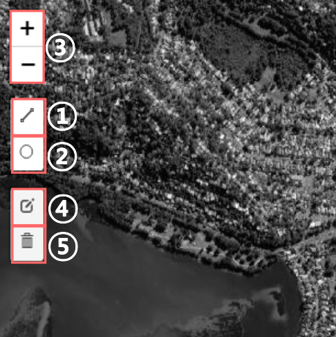
Fig. 3-1-3-2-1. Transect generation tools numbered as listed below.

1. Select the polyline tool. Click once to create points for the baseline from which the transects will extend. Draw the baseline close to the mapped shorelines on the landward side without overlapping with the shorelines. Double-click or click Finish to save the baseline.

2. Select the circle marker tool and click once on the ocean near the center of the beach to indicate the seaward direction. The transects will be automatically generated after both features are placed.

3. Click the Zoom in/out tools at any point to zoom in or out on the map.

Before transects are generated, you can also:

4. Select the edit tool to click on and move the baseline or circle marker.

5. Select the delete tool to click on and delete the baseline or circle marker.

Fig. 3-1-3-2-2 shows the results generated for Tairua Beach, New Zealand when the distance between transects is 200 meters and the transect length is 500 meters. To view the shoreline position over time for any of the given transects, the user can click on the desired transect on the map.

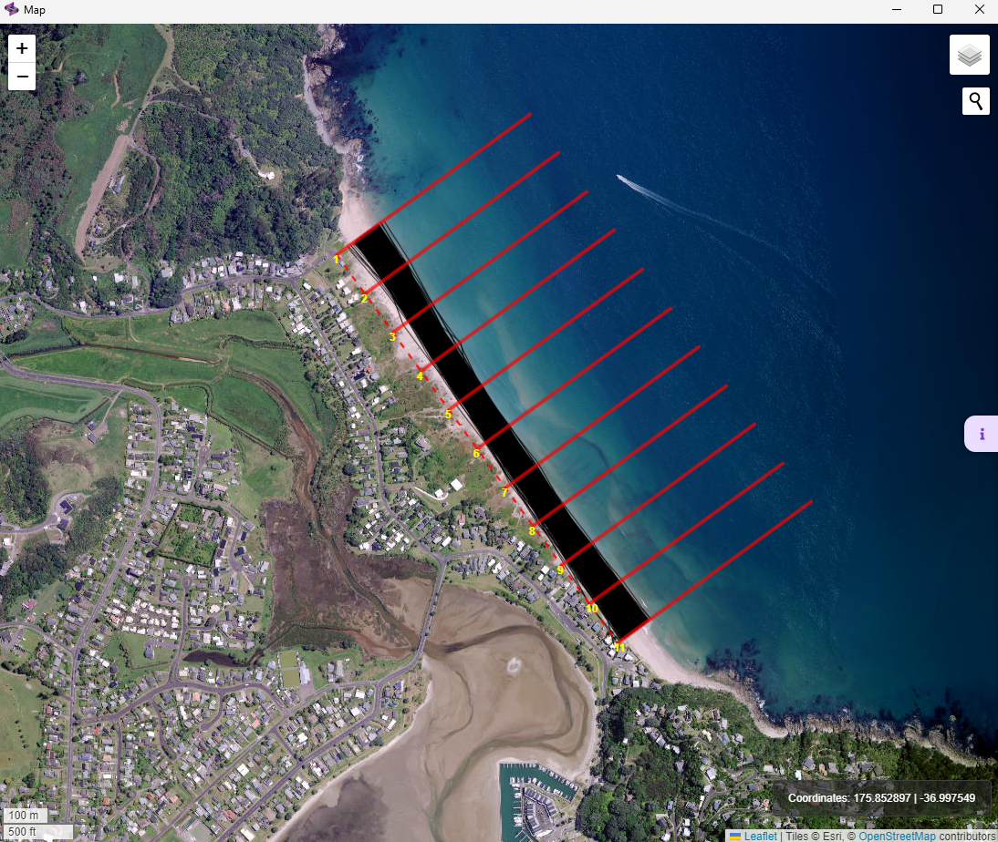Fig. 3-1-3-2-2. Example of transects generated for Tairua Beach, New Zealand.

Once the transects are generated on the map, the transects will be automatically saved and the window can be closed. The resulting numerical domain can be viewed again after closing the map by clicking “View current domain” at the bottom of the file tree.

3.1.3.3. Save Output

As the datasets are inputted into the Preprocess module, a variety of graphs will be automatically generated to display the data, as discussed in the next section. These graphs will be listed in the file tree on the left side of the Preprocess interface and can be viewed by clicking once on the graph’s title. Once all required data is inputted, the Save Output button will appear on the left side under the file tree. The user can then click this button to generate and save the NetCDF to the selected location in the File Navigator.

3.1.4. Output graphs and dataset

There are two main outputs resulting from the Preprocess module: graphs representing the inputted data and a NetCDF file containing the merged and preprocessed datasets. The contents of these outputs are described in the following sections.

3.1.4.1. Generated graphs

As the input files are selected and uploaded into the Preprocess module, several graphs are generated to better view and understand the data. This includes plots for wave forcing, tide and surge, and shoreline observations. All graphics generated can be saved for future use and reference once opened from the file tree.

Wave Forcing Graphs

Once wave forcing data is inputted, four plots are generated to represent the significant wave height, peak wave period, and wave direction in different forms. To better view these plots, the user can use the tools in the toolbar at the top of each graph to zoom in and out and modify the axes.

Significant Wave Height (Hs) Rose: Wave roses are a common way to represent both significant wave height and peak wave period and their respective dominant directions. As shown in Fig. 3-1-4-1-1, the base shape for this graphic is a circle divided into segments representing the primary cardinal directions. Sectors of the circle are then highlighted, with the longer segments representing a larger density of measurements in the covered range of directions. The legend then indicates the distribution of significant wave heights in meters within each sector. From Fig 3-1-4-1-1, it can be seen that the dominant wave direction is East, with most waves between 1.0 and 1.5 meters.

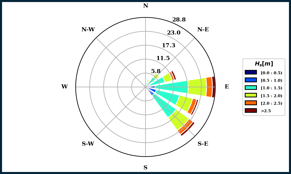Fig. 3-1-4-1-1. Example of Hs Rose generated for Angourie Back Beach, Australia.

Peak Wave Period (Tp) Rose: Similar to the Hs Rose, this graph indicates the distribution of Tp measurements in seconds within the range of directions indicated by each sector of the circle. From Fig. 3-1-4-1-2, it can again be observed that the dominant wave direction is East, with most waves having a measured Tp between 9.0 and 12.0 seconds.

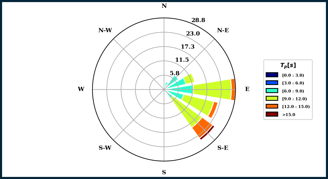Fig. 3-1-4-1-2. Example of Tp Rose generated for Angourie Back Beach, Australia.

Hs and Tp Density Plot: This plot represents which ordered pair of Hs and Tp values for any one wave are the most common when written in (x,y) form. As seen in Fig. 3-1-4-1-3, Hs values are plotted on the x-axis with their corresponding Tp values on the y-axis. The legend on the right side then indicates the number of values at any point, with the highest density appearing dark red and the lowest density appearing dark blue. From Fig. 3-1-4-1-3, we can see that the largest number of waves have a significant wave height of around 1.2 meters and a peak wave period of around 9 seconds, as indicated by the dark red spots on the graph.

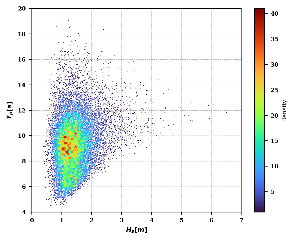Fig. 3-1-4-1-3. Example of Hs and Tp Density Plot generated for Angourie Back Beach, Australia.

Wave Time Series: These graphs represent the Hs measurements in meters, Tp measurements in seconds, and wave direction (Dir) measurements in degrees over time for the entire dataset, as seen in Fig. 3-1-4-1-4.

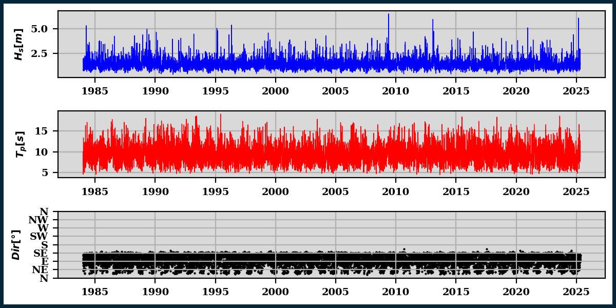Fig. 3-1-4-1-4. Example of Wave Time Series plots generated for Angourie Back Beach, Australia.

Tide and Surge Graphs

To represent the tide and surge data, two graphs are generated in the Preprocess module, including a time series plot and a histogram for each dataset.

Tide and Surge Time Series: In these plots, the tide or surge measurements in meters are plotted over time for the entire dataset, as seen in Fig. 3-1-4-1-5.

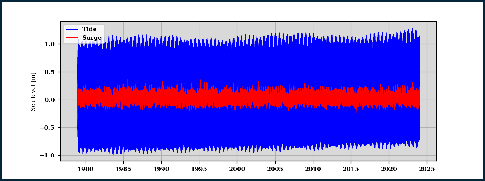Fig. 3-1-4-1-5. Example of Sea Level Time Series plots generated for Angourie Back Beach, Australia.

Tide and Surge Histogram: This graph acts as a representation of the density of tide and surge measurements independently. With the sea level measurement in meters on the x-axis, the density for a range of sea level measurements is plotted on the y-axis as a bar. The density value is the percentage of data points falling within the range that the bar spans on the x-axis. The bars plotted are also accompanied by a curve of best fit, serving as the density function for the dataset, as shown in Fig. 3-1-4-1-6.

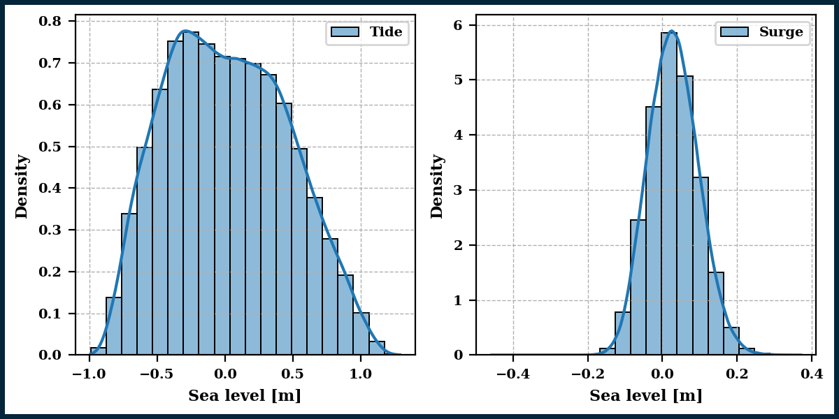Fig. 3-1-4-1-6. Example of Sea Level Histogram plots generated for Angourie Back Beach, Australia.

Shoreline Observation Graphs

Similar to the Tide and Surge data, time series plots and a histogram are generated for the Shoreline Observation data.

Shoreline Position Time Series: In this plot, the shoreline position measurements in meters are plotted over time for the entire dataset for each of the transects, as seen in Fig. 3-1-4-1-7. The color of the transect corresponds to the number of the transect, as indicated by the legend at the top of the plot.

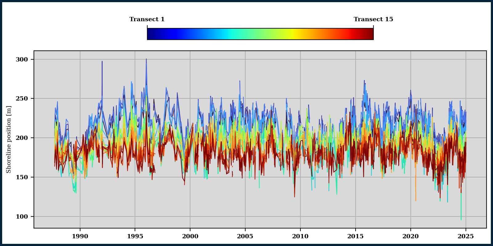Fig. 3-1-4-1-7. Example of the Shoreline Position Time Series plot generated for Angourie Back Beach, Australia.

Shoreline Position Histogram: This graph represents the density of shoreline position measurements on the y-axis for a range of measurements in meters as indicated on the x-axis. The bars plotted are also accompanied by a density function, as shown in Fig. 3-1-4-1-8.

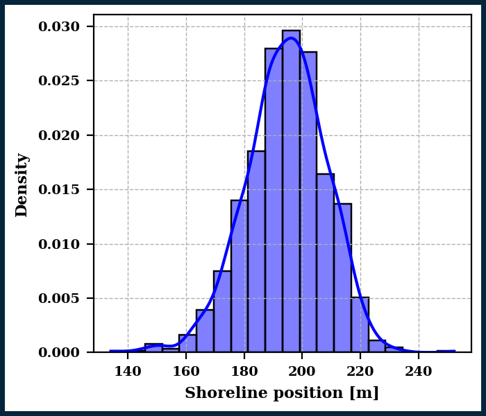Fig. 3-1-4-1-8. Example of the Shoreline Position Histogram generated for Angourie Back Beach, Australia.

Principal Component Analysis (PCA): This final graphic poduced is a PCA of the nearshore processes driving beach evolution (Fig. 3-1-4-1-9). It consists of two plots showing how the dominant modes of transport contribute to the observed shoreline variablity. More information about this method of analysis can be found in Blossier et al. (2015) and Jaramillo et al. (2021a).

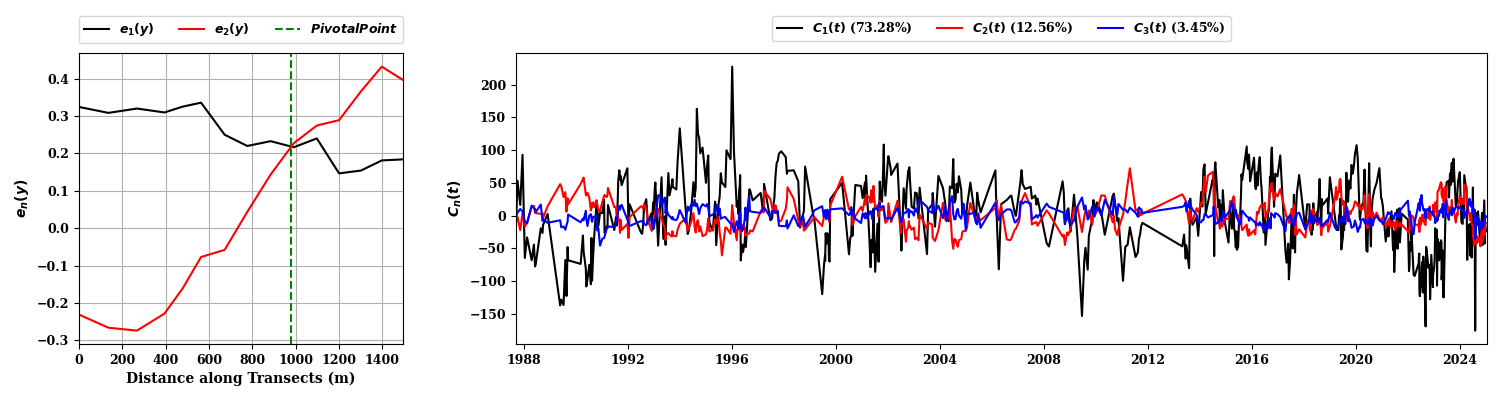Fig. 3-1-4-1-9. Example of Wave Time Series plots generated for Angourie Back Beach, Australia.

3.1.4.2. NetCDF file

Once the required input datasets are selected, the user will have the ability to generate and save the output NetCDF (.nc) file, providing a structured format for the variables essential for further modeling. The output file includes four subsections of data:

Coordinates: Coordinate and time data collected and processed from the wave forcing and shoreline observation datasets. This subsection of data includes the following variables:

Variable	Type	Units	Description
`time`	datetime64[ns]	–	Datetimes associated with each wave forcing data point
`lat`	float64	degrees north	Latitudes of waves
`long`	float64	degrees east	Longitudes of waves
`ntrs`	int32	number of	Numbered labels for transects.
`time_obs`	datetime64[ns]	–	Datetimes associated with each shoreline observation data point
`xi`	float64	meters	Initial x-values for transects
`yi`	float64	meters	Initial y-values for transects
`xf`	float64	meters	Final x-values for transects
`yf`	float64	meters	Final y-values for transects
`phi`	float64	degrees	Transect angle
`lat_waves`	float64	degrees north	Latitude of provided waves
`lon_waves`	float64	degrees east	Longitude of provided waves
`x_pivotal`	float64	meters	Initial x-coordinate of pivotal transect
`y_pivotal`	float64	meters	Initial y-coordinate of pivotal transect
`phi_pivotal`	float64	degrees	Angle of pivotal transects

Data Variables: Wave forcing, shoreline observation, and local sea level data associated with the times and coordinates defined in the Coordinates subsection. This subsection of data includes the following variables:

Variable	Corresponding Variables	Type	Units	Description
`hs`	(`time`,`ntrs`)	float64	meters	Significant wave height
`tp`	(`time`,`ntrs`)	float64	seconds	Peak wave period
`dir`	(`time`,`ntrs`)	float64	degrees north	Direction of wave propagation
`tide`	(`time`,`ntrs`)	float64	meters	Astronomical tide
`surge`	(`time`,`ntrs`)	float64	meters	Storm surge
`slr`	(`time`,`ntrs`)	float64	meters	Sea level rise
`obs`	(`time_obs`,`ntrs`)	float64	meters	Observed shoreline position
`rot`	(`time_obs`)	float64	degrees	Shoreline rotation
`average_obs`	(`time_obs`)	float64	meters	Average shoreline position
`mask_nan_obs`	(`time_obs`,`ntrs`)	bool	boolean	Mask for NaNs in shoreline observations
`mask_nan_rot`	(`time_obs`)	bool	boolean	Mask for NaNs in rotation
`mask_non_average_obs`	(`time_obs`)	bool	boolean	LMask for NaNs in average observations

Indexes: PandasIndex for each of the variables listed in the Coordinates subsection.
Attributes: List of contributions, sources, and conventions used in the Preprocess module to create the output file. This subsection of data includes the following attributes:

Attribute	Description
`title`	“Input File for IH-SET models”
`institution`	“Environmental Hydraulics Institute of Cantabria - https://ihcantabria.com/”
`source`	“IH-SET preprocessing module”
`history`	States the date created
`references`	“Jaramillo et al. (2025) - doi: xxxxxxxx.xx”
`Documentation`	“https://ihcantabria.github.io/IHSetDocs/”
`Conventions`	“CF-1.6”
`Data Sources`	Lists the file type of each input file used
`Summary`	“This dataset is output from the IH-SET preprocessing module. Etc…”
`geospatial_lat_min`	“-90”
`geospatial_lat_max`	“90”
`geospatial_lon_min`	“-180”
`geospatial_lon_max`	“180”
`applicable_models`	Lists the models that can be applied to the data included in the output file.
`EPSG`	States the European Petroleum Survey Group (EPSG) coordinate code for the latitude and longtitude data

Fig. 0