4. Test Cases
Along with the IH-SET software, test cases are provided for download:
Case 1 - Curl Curl Beach: New South Wales province, Australia.
Case 2 - Tairua Beach: West coast of the North Island of New Zealand.
Figure 4 shows the location of the test cases on the map.
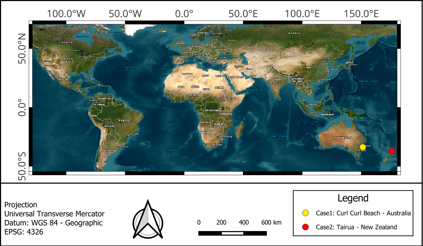
Fig. 4. IH-SET test cases locations.
4.1. Introduction to Study Sites
Both study sites serving as the bases for the provided test cases are located in the southwest Pacific, though they have differing characteristcs that make them suitable examples for the IH-SET software. This section discusses some of the key features of these beaches.
4.1.1. Case 1: Curl Curl Beach, Australia.
The stretch of beach at Curl Curl is divided into North and South Curl Curl beaches in the same beach arc. Curl Curl beach is known for having some of the best surfing spots in the Northern Sydney suburbs of the province of New South Wales, Australia (Fig. 4-1-1-1).
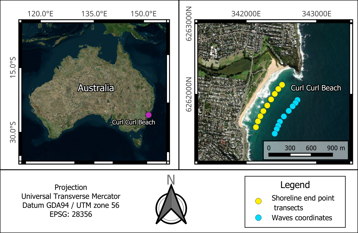
Fig. 4-1-1-1. Location, shoreline example, and Wave Points locations for the Curl Curl beach that can be freely accessed in the GitHub of ShoreShop 2.0: Comparative Study of Shoreline Models (Case 1).
Beach Morphology: Curl Curl Beach has a 1.2 km long highly exposed shoreline, with a NE-SW orientation and a SE-facing beach arc. The typical average slope (β) ranges between 0.05 and 0.1 m/m.
Waves: The deep-water wave climate is considered of high wave energy, where the mean Hs ≈ 1.2 m and Tp ≈ 9.04 s, while the wave incidence direction is dominated by long-period persistent swell from a SE direction (Fig. 4-1-1-2).
Tides: The Curl Curl tidal regime is microtidal and semidiurnal with a mean spring tidal range of around X2 m (Fig. 4-1-1-3).
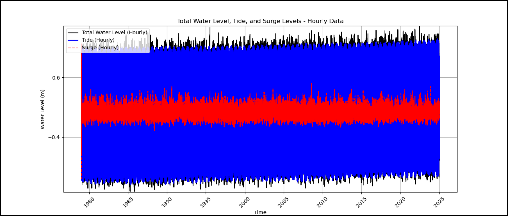 Fig. 4-1-1-2. Curl Curl Beach tides and storm surge from CODEC-ERA5 Copernicus Global Tide Model.
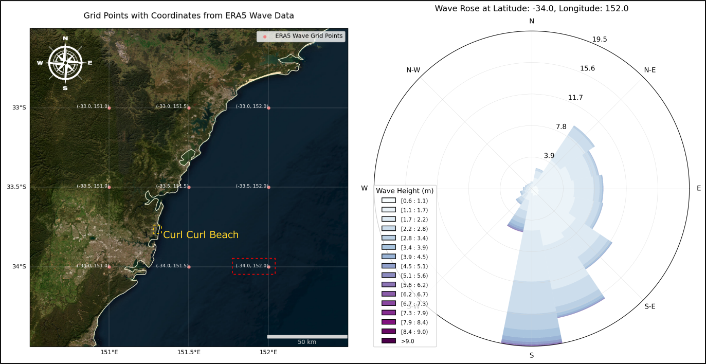 Fig. 4-1-1-3. Curl Curl Beach deepwater wave climate from ERA5 Global Wave Model.
Curl Curl Beach Dataset (Download)
ShoreShop 2.0:
Advancements in Shoreline Change Prediction Models
Benchmarking shoreline prediction models over multi-decadal timescales
https://www.nature.com/articles/s43247-025-02550-4
Original INPUT Datasets:
https://zenodo.org/records/15259391
IH-SET formatted dataset (ready to use):
sha256:e9a7a1b9c4986a1271c2c77ecac522686bf6b3876cf57028049138a25d43f817
4.1.2. Case 2: Tairua, New Zealand.
Tairua Beach is located on the east coast of the Coromandel Peninsula in the North Island of New Zealand (Fig. 4-1-2-1).
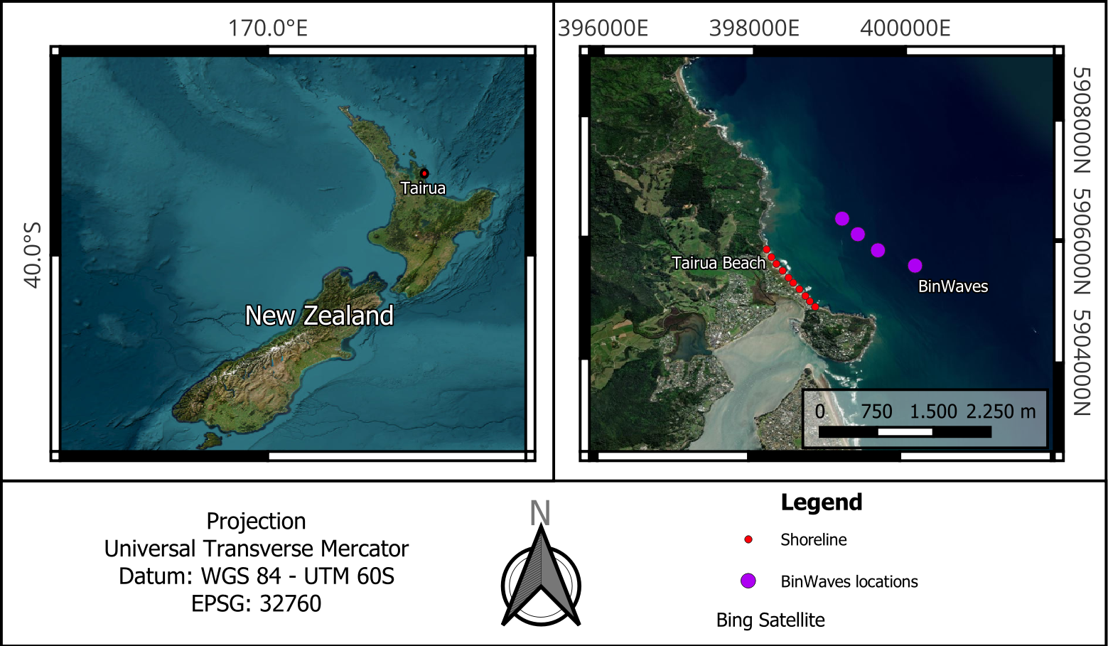
Fig. 4-1-2-1. Location, shoreline example, and BinWaves locations mapped for the Tairua study site (Case 2).
Beach Morphology: Tairua Beach presents morphodynamic characteristics dominated by Reflective Bar Beach. The orientation of Tairua Beach is predominantly NW-SE, with a normal direction close to 53° (NE). The beach profiles are generally steep and characterized by medium-coarse sand, with a slope (β) of 0.13.
Waves: The Tairua deep water wave climate is moderate to high wave energy, with Hs range of 0.1 - 4.4 m and Tp varying from 2.2 - 22.1 s. The mean Hs is ≈0.7 m, Tp ≈ 10 s and dominante wave direction is E - NE (Fig. 4-1-2-2).
Tides: The Tairua tidal regime is microtidal and semidiurnal, with a tidal range of up to 2 m (Fig. 4-1-2-3).
 Fig. 4-1-2-2. Tairua tides and storm-surge from CODEC-ERA5 Copernicus Global Tide Model.
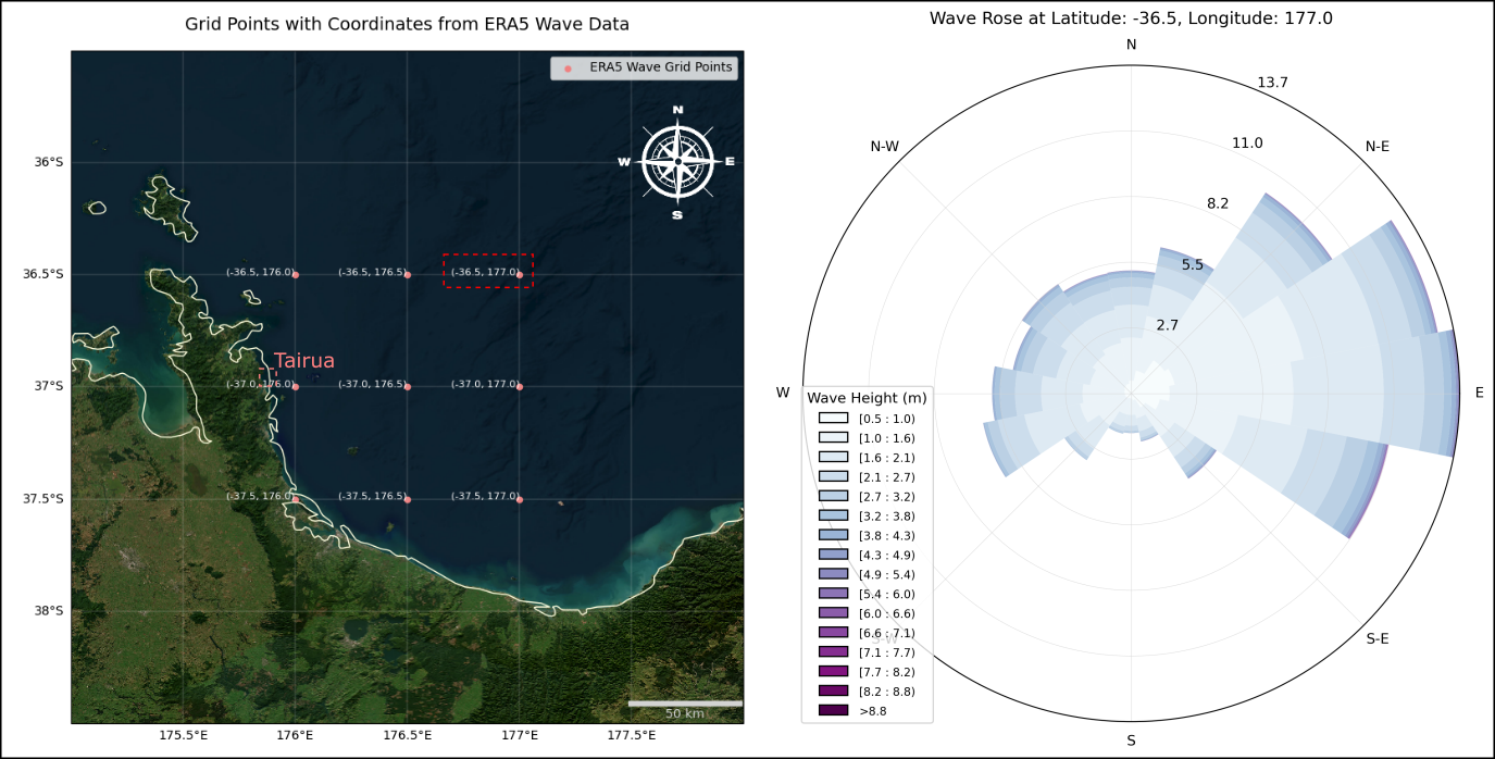 Fig. 4-1-2-3. Tairua deepwater wave climate from ERA5 Global Wave Model.
Tairua Beach Dataset (Download)
ShoreShop 1.0:
SHORECASTS: A blind-test of Shoreline Models
https://www.worldscientific.com/doi/epdf/10.1142/9789811204487_0055
Original INPUT Datasets: ShoreShop (Montaño et al., 2020) - available on the University of Aukland website.
IH-SET formatted dataset (ready to use):
sha256:a76b0fa3891d7e46072c6ed18abc64e0551f61caea609c284ae5e82eb413bd44
4.2. Input Files Examples
4.2.1. Wave Files:
The input files to be loaded into the Preprocess module to generate the NETCDF in the IH-SET standard are plain text files in CSV format.
IH-SET accepts time series for a single point or for multiple wave points near the surf zone or beach closure profile. For cases involving multiple wave points, it is important to name the input CSV files with the same base name, but numbering the end of the file names according to the order of the associated beach profiles, as in the example below in a beach with 15 beach profiles and 15 wave points:
Suggested name for wave files according to transect association:
nearshore_waves_timeseries_transect_01.csv
nearshore_waves_timeseries_transect_02.csv
nearshore_waves_timeseries_transect_03.csv
…
nearshore_waves_timeseries_transect_15.csv
The data in each CSV should have a header with the variable names as in the example below, using the first 10 lines of one of the input CSVs:
nearshore_waves_timeseries_transect_01.csv content:
time,Hs,Tp,Dir
1940-01-02,0.955587402,7.489383124,116.8650704
1940-01-03,0.986981874,5.479013276,87.80441075
1940-01-04,1.426444472,6.420172485,73.51347322
1940-01-05,1.248591206,6.801605915,70.22703469
1940-01-06,0.705501012,6.950942889,79.88670194
1940-01-07,1.146077182,5.482588834,125.5313966
1940-01-08,1.131035458,5.721648541,127.1965788
1940-01-09,0.840004178,6.829882205,109.2263848
1940-01-10,0.843138868,7.927856374,99.3055916
...
In addition to the file(s) containing the wave time series data, it is essential to provide the file with: (a) the coordinates of the wave point(s) (X,Y); (b) the estimated depth of the wave point(s); and (c) the definition of the project’s coordinate system in EPSG code, as shown in the example below:
Coordinate file: nearshore_waves_coords.csv:
lon,lat,depth,epsg
342728.49839001364,6261920.365477566,15,32756
342701.13906130445,6261878.3398511065,15,32756
342660.3934545089,6261831.219421092,15,32756
...
342604.74627520185,6261766.866004263,15,32756
Note: For projects with a single wave point near the beach of interest, the wave point coordinate file is not necessary; the single point information can be entered directly into the auxiliary pop-up window that opens immediately after loading just one CSV wave file, as shown in Figure 4-2-1 below.
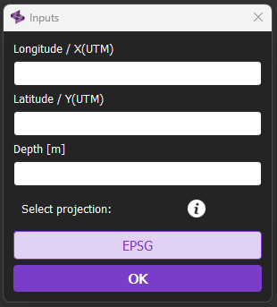
Fig. 4-2-1. Pop-up window for entering location data for the single time series of wave data.
4.2.2. Tide and Surge Files:
Similar to wave data, tidal data can be provided as a time series of water level oscilation in the area of interest. Either one file containing a time series of tides measured by tide gauge or by global astronomical tide models can be provided, or two files can be provided, with the second containing storm surge data complementing the first astronomical tide file.
The examples below show the formatting of the astronomical tide and storm surge files with their respective headers for the Preprocess module to recognize the tidal input data.
Astronomical tide file: tide_timeseries.csv
time,tide
1950-01-01,0.01031358994119
1950-01-02,-0.0001428425773902
1950-01-03,-0.0081518937384059
1950-01-04,-0.0166269009864276
1950-01-05,-0.0236500053011406
1950-01-06,-0.0268531034303317
1950-01-07,-0.0244905341298127
1950-01-08,-0.0163098156375265
1950-01-09,-0.003733772358122
...
Storm surge file: stormSurge_timeseries.csv
time,surge
1979-01-01 00:00:00,0.129
1979-01-01 01:00:00,0.594
1979-01-01 02:00:00,0.96
1979-01-01 03:00:00,1.16
1979-01-01 04:00:00,1.136
1979-01-01 05:00:00,0.947
1979-01-01 06:00:00,0.491
1979-01-01 07:00:00,0.026
1979-01-01 08:00:00,-0.489
...
4.2.3. Shoreline Files:
The provided coastline file must contain the time series for each beach profile as a comma-separated field in a CSV file, where each line corresponds to the distance of the coastline on the measured date relative to a “zero” reference point. That is, if transect 1 on the first date has a value of 100, it means the coastline was 100 m from the zero reference point; if on date 2 it was 90 m, it means there was 10 m of erosion, with the coastline receding 10 m. Similarly, the file should present this information for beach profiles 2, 3 up to profile “N” for “n” measurements in the time series, as shown in the example below:
time,Transect1,Transect2,Transect3,Transect4,Transect5,Transect6,Transect7,Transect8,Transect9
1999-02-17,197.0257945,192.9696576,194.3851155,196.5707127,203.4011533,207.9024136,206.3231592,199.5021462,193.6885209
1999-03-05,185.473336,186.2792623,184.12346,181.0004045,206.6121929,198.4735871,205.9505909,195.0288654,180.2099104
1999-06-25,203.434419,198.0199997,190.3943878,187.1033692,174.7376758,175.5412808,171.384529,167.0836541,181.9392211
1999-07-11,199.7269429,203.2526594,196.1392681,183.3788671,187.8351724,183.2480251,179.708851,170.7768308,184.3490052
1999-07-19,198.3141951,192.1924483,194.4845273,188.2955083,184.8517458,181.9164998,181.8491385,166.1814958,175.3513967
1999-07-27,190.8534258,185.5487653,189.6832994,191.1443615,180.2208572,181.6202349,178.0131711,165.9552856,173.7703447
1999-08-04,198.7494417,195.06571,201.742722,196.5505113,190.1980939,182.4724258,182.3011521,171.2001507,
1999-08-12,203.0815256,200.3315556,205.7858809,197.6515397,197.2535933,194.7883334,198.1869158,182.6968171,195.8827032
1999-08-20,197.4463953,196.97335,195.7287974,197.3591001,192.2584477,191.9580283,192.853369,184.5928018,182.750933
...
n
The coastline time series file requires a supplementary file with the initial and final coordinates of each beach profile present in the coastline time series file. This file must contain (a) the initial and final X,Y positions of each beach transect; along with (b) the EPSG code of the coordinate system adopted for the transects, which must necessarily be in a Cartesian system (UTM) with shoreline displacement in meters. (Note: Do not use a geographic coordinate system in degrees for the shorelineline positions!)
xi,yi,xf,yf,epsg
342225.9226699482,6262416.651688941,342510.5207102382,6262135.6152648935,32756
342145.86837244686,6262327.809567636,342456.75336726283,6262076.160429122,32756
342078.2955608561,6262234.958167378,342406.9449423171,6262007.009413937,32756
342019.63594314636,6262146.579776522,342355.1556159202,6261928.840602154,32756
341966.9109116632,6262063.512634694,342300.6208924615,6261843.08331215,32756
341908.2964570696,6261978.129101633,342245.9826764337,6261763.646552926,32756
341850.0128006046,6261878.441514831,342203.18732838973,6261690.727917372,32756
341798.4472587181,6261770.323785321,342168.52929537644,6261618.720127417,32756
341762.1118180726,6261665.564159464,342140.352577665,6261535.727098524,32756
These text files must be prepared in the formats indicated above to be added to the Preprocess module in order to generate the final NetCDF input file for the IH-SET model. Note: Do not provide files with the string “Nan” for fields without data; simply use the empty field format. Do not fill anything between commas!
Example of a row with all the data filled in:
2001-11-29,191.9171292,190.2146202,195.0066272,186.2494232,184.5732751,193.5067476,190.9692881,185.9322233,192.499361
Example of a row with partially empty data:
2001-12-31,,,,,,,181.3759199,186.7448735,182.1501864
4.3. Other Data Sources
Regardless of the data source used as input for the IH-SET models, the formats of the input CSVs must always comply with the formatting described in item 4.2. Input Files Examples.
4.3.1. Wave data
The European Centre for Medium-Range Weather Forecasts (ECMWF) ERA5 hourly data on single levels from 1940 to present reanalysis database. ERA5 provides hourly estimates for a large number of a ocean-wave parameters updated daily with a latency of about 5 days, which can be accessed via the link:
An overview of all ERA5 datasets can be found in this link.
Wave files can be downloaded in NetCDF format separated by days, months or years, for regular grids with 0.5 degree resolution on the Climate Data Store (CDS) page, which include detailed manuals on how to download the reanalysis data for any region of the world.
The Global Ocean Waves Reanalysis (WAVERYS) database from the Copernicus Marine Service.
The WAVERYS database provides a single NetCDF file with data with a 3-hour frequency since 1980 in a grid resolution of 1/5 degree.
There are detailed PDF manuals for accessing the data from the Copernicus Marine Service database.
Both databases can be downloaded by code via Python API.
Additionally, the wave data extracted was propogated to multiple points in shallower water using the BinWaves methodology developed by Cagigal et al. (2024). The first step in this methodology is the generation of a library of monochromatic offshore wave cases sorted into directional bins with a defined propogation coefficient. After creating this library, the propogated wave spectra can be generated for each bin using linear energy superposition to a nearshore location. This method is applied in the BlueMath toolkit developed by the GeoOcean group at the Universidad de Cantabria. By applying this methodology, propogated wave data for multiple nearshore points could be generated, allowing for more accurate simulations of shoreline evolution along the beaches.
4.3.2. Tide data
The FES2022 (Finite Element Solution) model, which is an astronomical global tide prediction model based on harmonic constants.
The FES2022 tides database includes two components: tide elevations (amplitude and phase) and tide loading (amplitude and phase) on a 1/30°x1/30° grid.
The FES2022 model user manual for downloading data can be found in PDF format.
The CODEC ERA5 - Global sea level change time series from 1950 to 2050 derived from reanalysis and high resolution CMIP6 climate projections. This dataset provides time series of global sea level related variables including tides, storm surges and sea level rise from 1950 to 2050 based on hydrodynamic modelling using the Deltares Global Tide and Surge Model (GTSM) version 3.0, with Coastal Grid points resolution of 0.1° and Reanalysis data frequency of 10-minute, hourly and daily maximum in NetCDF-4 format.
Tidal reanalysis data for total water level and storm surge variables from 1940 to the present can be downloaded from the link:
The procedures for downloading CODEC data for any region of the world are the same as for downloading WAVE data from the CDS ERA5 model.
4.3.3. Shoreline data
Coastline time series for Angourie were extracted with the CoastSat Space application developed by Vos et al. (2019).
CoastSat is an open-source software toolkit written in Python, connected to the Google Earth Engine servers to process multispectral satellite images from the Landsat-5, 7, 8 and 9 and Sentinel-2 missions, that enables users to obtain time-series of shoreline position at any coastline worldwide from 40 years (and growing).
The CoastSat application detailed manual and example scripts for executing the code in the project’s Github repository.
Historical, up-to-date shoreline data dervied from the CoastSat toolbox are available for Australia, Japan, and parts of North and South America on the CoastSat Space website, from which these test cases were extracted.
The time series for Tairua were sourced form the Cam-Era program at Tairua Beach, involving computer-controlled video cameras that monitor the environment for data collection and research. The Cam-Era program is maintained by NIWA, the National Institute of Water and Atmospheric Research of New Zealand. The Tairua Camera has operated from August 1997 to present. Every hour during daylight time, 600 images (one every second for 10 minutes) are taken. The first of the 600 is saved as an individual image before the total 600 images are averaged and saved as one image available on the NIWA web site.
Figure 4-2-3-1 shows the camera image from March 18th 17:30 (NZST) for Tairua Beach.
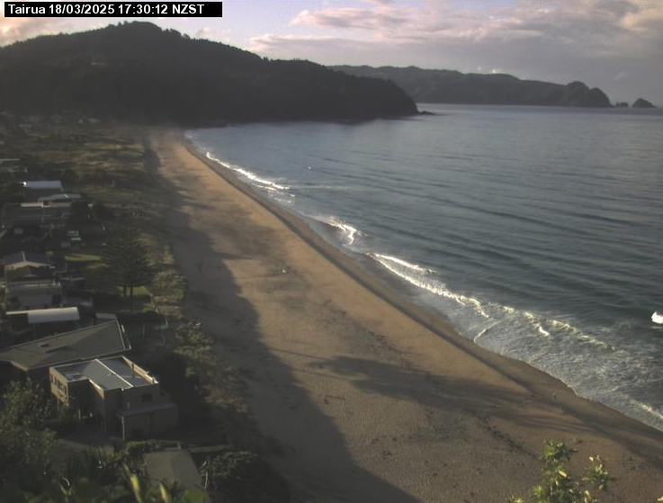
Fig. 4-3-3-1. Tairua Beach camera image from March 18th 17:30 (NZST).