Davidson et al. (2013)
Description
Davidson et al. (2010) presented a model based on the disequilibrium concept introduced by Wright et al. (1985), which suggests that the beach state correlates with the dimensionless fall velocity and that the future beach state is affected by antecedent values of this parameter. However, this original model neglected any dependence on the equilibrium of antecedent shoreline conditions, leading to difficulties predicting the direction of shoreline change. To account for this, Davidson et al. (2013) considered that future shoreline positions can depend on past morphodynamic and hydrodynamic conditions with some lag, suggesting a model for shoreline evolution (ShoreFor) as follows:
\(P\) : the incident wave power
\(Ω\) : the time-varying dimensionless fall velocity (\(Ω=H/w_sT\))
\(Ω_{eq}\) : the weighted average of the antecedent dimensionless fall velocity
\(b,c^±\) : the free parameters where \(c^+\) indicates the accretion and \(c^-\) indicates the erosion, respectively
The primary revision to the Davidson et al. (2010) model was the addition of a time-varying equilibrium condition within the disequilibrium term. This time varying-equilibrium condition is defined as the weighted average of the antecedent dimensionless fall velocity controlled by a memory decay parameter (ϕ), which is related to the dominant time-scale of shoreline variability, as presented below:
\(ϕ\) : the memory decay of the system
\(D\) : the total window width of the weighted average
It was determined that this model is suitable for application in microtidal to mesotidal, energetic, exposed sandy beaches where cross-shore transport processes dominate. While designed for use over time scales spanning several years to decades, the model demonstrated skill in hindcasting shoreline variability observed weekly over multiple years, suggesting this approach may be suitable for a wider range of applications.
Simulation procedure
The following describes the procedure for simulating the Davidson et al. (2013) model. The figure below illustrates the start screen for simulating the model.
Upload the required file (see NetCDF file in Simulation inputs below) using the Browse File button in the Models tab.
Select the desired model from the list of modules to open the model’s start screen.
Adjust the input parameters and simulation settings in the side panel according to the model’s requirements (see Calibration settings in Simulation inputs below).
Click on the “Run Model” button to start the model execution.
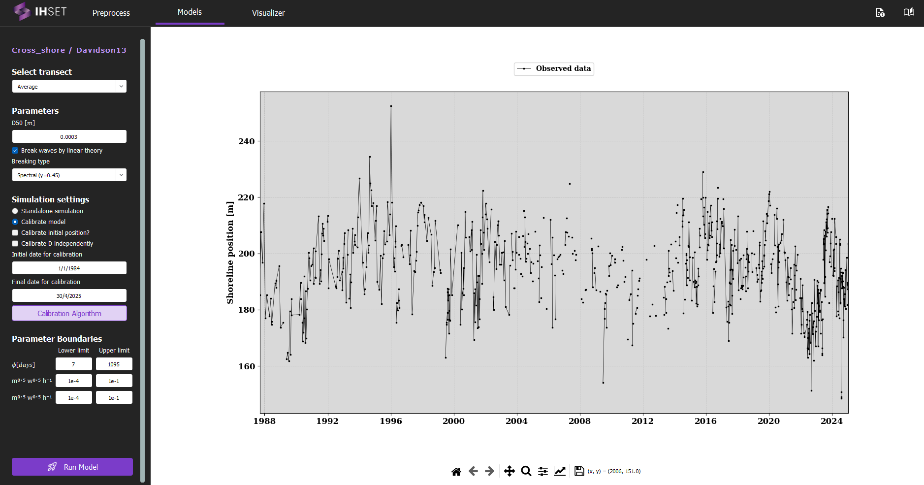
Fig. 3-3-1-3-1. Start screen for simulating the Davidson et al. (2013) model.
Simulation inputs
This section outlines the input file, parameters, and simulation settings necessary to run this model in accordance with the procedure provided in the previous section.
NetCDF file
The primary input to run the Davidson et al. (2013) model is the NetCDF file produced using the Preprocess module. More information about the contents of this dataset can be found here. This file provides the wave forcing data, comprised of wave data and optionally sea level data, which is inputted directly into the equations for the model. The NetCDF also contains the shoreline observation data, which is used to calibrate the model. For more information about the calibration process and parameters, please check the Calibration section.
As mentioned in the Simulation Procedure, this file is inputted in the Module tab prior to selecting the model. Once the required data for simulation is added and the model is selected, the screen transitions to the view shown in Fig. 3-3-3-1 above.
Parameters
In addition to the NetCDF file provided, a number of parameters must be entered into the module on the left side of the interface. These parameters are assumed to be constant over time and are included as constants in this model as follows:
D50 \([m]\) : Median grain size (Range : [0 ~ 2.0e-3])
If “Break waves by linear theory” is selected, the user will have the option to select the Breaking type (spectral or monochromatic), which determines the breaker index (\(γ\)) used.
Calibration Settings
Finally, the simulation settings and parameter boundaries must be selected for calibration. In the side panel, the user can decide to run a standalone simulation or to calibrate the model, described as follows:
Standalone simulation: The model is run with no calibration required, as the date range and parameter values will be entered manually. The options to use the first observation as the initial shoreline position (\(Y_0\)) and to use \(D=2Φ\) will also be given. Otherwise, these values must be entered manually.
Calibrate model: As opposed to the standalone simulation, this will run the model with calibration. The user can then decide whether or not to calibrate the initial position, \(Y_0\), and to calibrate D independently.
When calibrating the model, the default initial and final dates for calibration will coincide with the start of the wave data and the end of the shoreline data respectively, though these values can be modified to better suit the data used and the desired output. It is important to note that that results for the ShoreFor model will always begin with a straight line resulting from the warm-up period for the convolution. For this reason, it is recommended that calibration begin a couple years before the shoreline observations.
The user also has the option to modify the calibration algorithm and the parameter boundaries. Though it is not necessary to modify these elements, doing so may can improve the performance or run time of the model.
Assimilation by Ensemble Kalman Filter (EnKF): The Ensemble Kalman Filter (EnKF) is a sequential data assimilation technique used to optimally combine model predictions and observations for dynamic, potentially non-linear systems. The EnKF represents the system state using an ensemble of realizations, allowing the estimation of statistical moments (mean and covariance) directly from the ensemble. Each realization is propagated forward using the model dynamics, and updated whenever observations become available.
The method consists of two main steps:
Forecast step:
Each ensemble member is propagated forward using the model:\[ \mathbf{x}_t^{(k)} = \Phi\left(\mathbf{x}_{t-1}^{(k)}\right) \]where \(\mathbf{x}_t^{(k)}\) is the state vector of ensemble member \(k\), and \(\Phi\) represents the (possibly non-linear) model operator.
Update step:
The ensemble is updated using observations \(\mathbf{y}_t\):\[ \mathbf{x}_t^{(k)} \leftarrow \mathbf{x}_t^{(k)} + \mathbf{K} \left( \mathbf{y}_t + \boldsymbol{\epsilon}_t^{(k)} - \mathbf{H}\mathbf{x}_t^{(k)} \right) \]where:
\(\mathbf{H}\) is the observation operator,
\(\boldsymbol{\epsilon}_t^{(k)}\) represents observation noise,
\(\mathbf{K}\) is the Kalman gain matrix.
The Kalman gain controls the balance between model predictions and observations and is defined as:
where:
\(\mathbf{C}_{xx}\) is the forecast state covariance estimated from the ensemble,
\(\mathbf{R}\) is the observation error covariance matrix.
Key characteristics:
Approximates mean and covariance using an ensemble of realizations.
Suitable for non-linear and high-dimensional systems.
Sequentially assimilates data as observations become available.
Can update both:
Model state variables
Model parameters (augmented state formulation)
Naturally incorporates uncertainty from both model and observations.
Application in IH-SET:
When enabled, the EnKF allows the model to assimilate observational data during simulations, dynamically correcting shoreline predictions and improving parameter estimation. This is particularly beneficial for systems with strong temporal variability and limited observational coverage.
Simulation results
Using the dataset provided along with the IH-SET software for Angourie Back Beach, Auatralia, running the model simulation yields several detailed outputs as shown in Fig. 3-3-1-3-2:
Comparison of Model Simulation Results and Observed Data: This shows the differences between the model’s shoreline position predictions and actual observed data over the simulation period.
Time-Series Variation of Forcing Variables: Displays changes in key forcing variables, such as wave climate and sediment transport, over time, providing context for the shoreline response.
Parameter Table Using Calibration Algorithm: Lists the parameters optimized for the model simulation, which are derived from calibration processes to enhance model accuracy.
Calibration and Validation Metrics: A table summarizing performance indicators such as RMSE (Root Mean Square Error), NS (Nash-Sutcliffe Efficiency), R² (Coefficient of Determination), and Bias, assessing the model’s predictive accuracy during both calibration and validation phases.
These outputs together provide a comprehensive view of model performance and reliability, allowing users to evaluate and interpret the shoreline evolution predicted by the simulation.
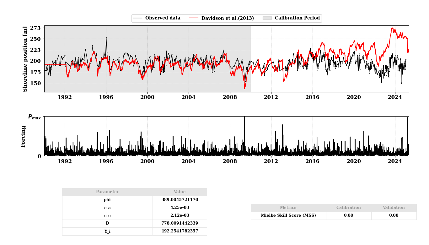
Fig. 3-3-1-3-2. Simulation results for Davidson et al. (2013).
In addition, several other functionalities enhance the usability of the model simulation interface:
“Save Results” Button: Allows users to save the simulation results to an output NetCDF file, enabling further analysis or documentation of the model output. All saved simulations can be viewed in the “Visualizer” to compare the results with other EBSEM models, facilitating a side-by-side evaluation of model performance. For more details, please check Visualizer
Other buttons: These buttons allow users to customize and adjust the figures related to the simulation results. Users can modify visual elements such as axis labels, graph types, or legends for clearer interpretation or presentation. Once the desired adjustments are made, users can save the figures in various formats for further use or reporting.
These features enable users not only to analyze and retain results but also to compare multiple models effectively for enhanced decision-making in shoreline evolution modeling.