Hanson and Kraus (1989)
Description
The one-line model is a long-term shoreline evolution model that calculates shoreline movements based on longshore sediment transport (LTS) gradients. The model is built with the assumption that the beach profile does not change with time in the long term. The model is suitable for sandy beaches with LST gradients over time.
The numerical domain is defined by a reference line and transects extending from this line towards the sea. While the transects and reference line are defined by their initial and final coordinates in any metric system, UTM coordinates are preferred to obtain the shoreline response in real-world coordinates. Fig. 3-4-1 presents a sketch of the one-line domain.
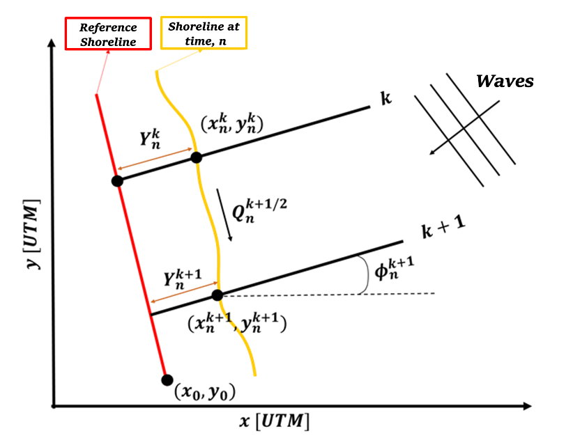
Fig. 3-4-1. Definition sketch of the one-line model proposed by Hanson and Kraus (1989).
The model proposed by Hanson and Kraus (1989) is formulated as follows:
\(y\) : cross-shore shoreline position at a given time [ \(m\) ]
\(t\) : time [ \(s\) ]
\(Q\) : longshore sediment transport (LST) [ \(m^3 s^{-1}\) ]
\(x\) : alongshore shoreline position [ \(m\) ]
\(q\) : sinks and sources along the coast [ \(m^2 s^{-1}\) ]
\(h^*\) : depth of closure [ \(m\) ]
\(h_{Berm}\) : berm height [ \(m\) ]
The LST in the original model is calculated using the CERC (1984) formulation, given by:
\(K\) : calibration parameter [ \(ms^{-1}\) ]
\(γ_b\) : breaker index [ \(-\) ]
\(ρ\) : density of water [ \(kg m^{-3}\) ]
\(g\) : acceleration due to gravity [ \(ms^{-2}\) ]
\(H_{s,b}\): significant wave height at breaking [ \(m\) ]
\(θ_b\): wave angle at breaking [ \(°\) ]
As previously mentioned, the category of model is used to estimate long-term average changes driven by longshore sediment transport and is not suitable for analyzing short-term changes, where cross-shore transport across the beach profile becomes relevant.
Simulation procedure
The following describes the procedure for simulating the Hanson and Kraus (1991) model. The figure below (Fig. 3-4-2) illustrates the start screen for simulating the model.
Upload the required file (see NetCDF file in Simulation inputs below) using the Browse File button in the Models tab.
Select the desired model from the list of modules to open the model’s start screen.
Adjust the input parameters and simulation settings in the side panel according to the model’s requirements (see Calibration settings in Simulation inputs below).
Click on the “Run Model” button to start the model execution.
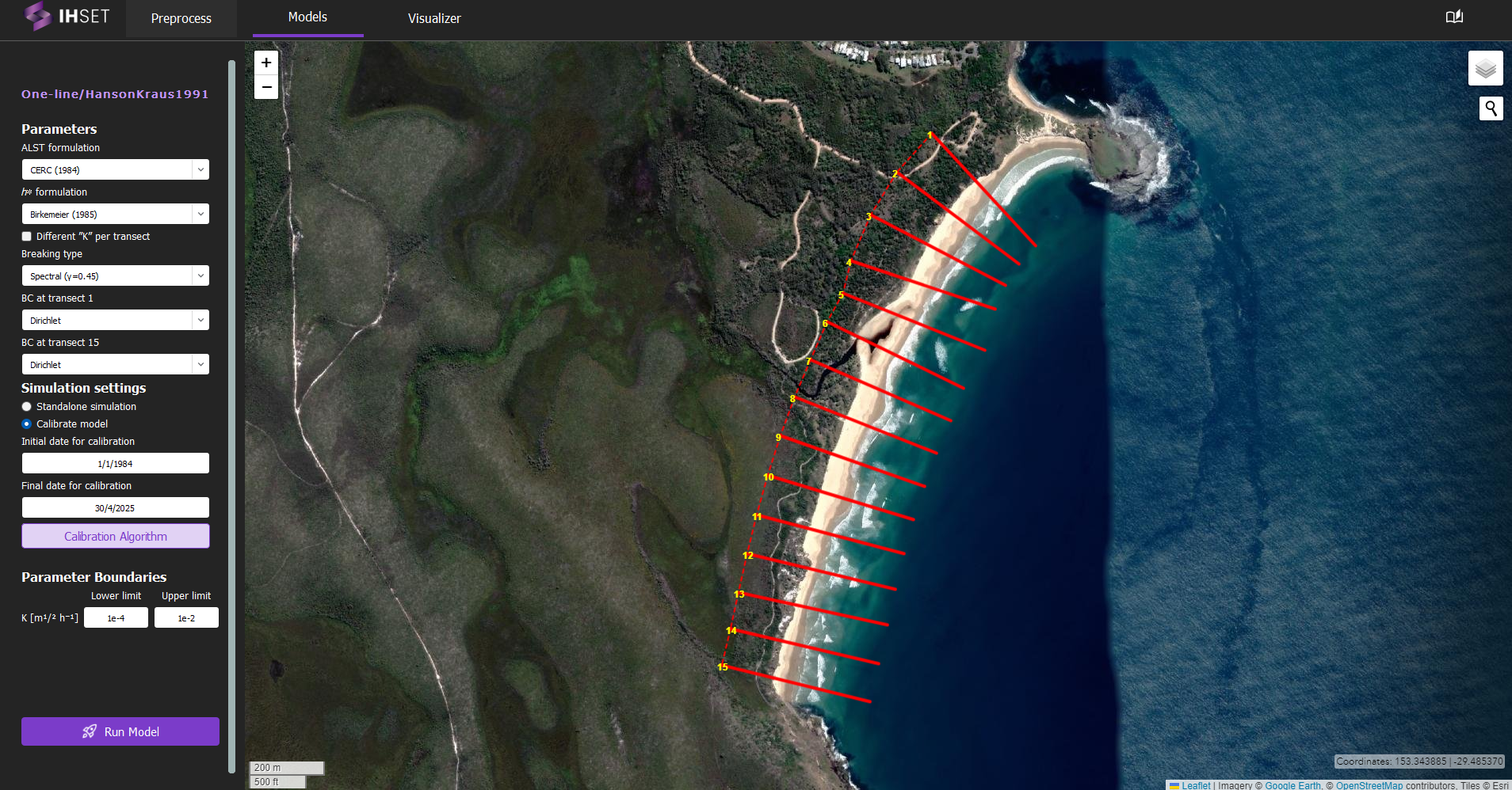 Fig. 3-4-2. Start screen for simulating the Hanson and Kraus (1991) model at Angourie Back Beach, Australia.
Simulation inputs
This section outlines the input file, parameters, and simulation settings necessary to run this model in accordance with the procedure provided in the previous section.
NetCDF file
The primary input to run the Hanson and Kraus (1991) model is the NetCDF file produced using the Preprocess module. More information about the contents of this dataset can be found here. This file provides the wave forcing data, comprised of wave data and optionally sea level data, which is inputted directly into the equations for the model. The NetCDF also contains the shoreline observation data, which is used to calibrate the model. For more information about the calibration process and parameters, please check the Calibration section.
As mentioned in the Simulation Procedure, this file is inputted in the Module tab prior to selecting the model. Once the required data for simulation is added and the model is selected, the screen transitions to the view shown in Fig. 3-5-2.
Parameters
In addition to the NetCDF file provided, a number of parameters must be entered into the module on the left side. These parameters are assumed to be constant over time and are included as constants in this model as follows:
LST Formulation: Formulation for LST. The user has the choice amongst CERC (1984), Komar (1998), Kamphuis (2002), or Van Rijn (1985).
\(h^*\) Formulation: Formulation used to calculate the depth of closure. The user has the choice between Birkemeier (1985) or Hallermeier (1978).
Different “K” per transect: Option to calibrate the calibration parameter “K” for each transect, rather than calibrating a sigular parameter across all transects.
Breaking Type: Formulation used to break waves (monochromatic or spectral)
BC at Transect 1: Boundary condition set for the first transect (Dirichlet or Neumann)
BC at Transect [final]: Boundary condition set for the final transect (Dirichlet or Neumann)
Calibration Settings
Finally, the simulation settings and parameter boundaries must be selected for calibration. In the side panel, the user can decide to run a standalone simulation or to calibrate the model, described as follows:
Standalone simulation: The model is run with no calibration required, as the date range for simulation and parameter values will be entered manually. The option to use the first observation as the initial shoreline position (\(Y_0\)) or to enter it manually will also be given.
Calibrate model: As opposed to the standalone simulation, this will run the model with calibration. The user can then decide whether or not to calibrate the initial position, \(Y_0\).
When calibrating the model, the default initial and final dates for calibration will coincide with the start of the wave data and the end of the shoreline data respectively, though these values can be modified to better suit the data used and the desired output. The user also has the option to modify the calibration algorithm and the parameter boundaries. Though it is not always necessary to modify these elements, doing so may improve the performance and run time of the model. Note that the parameter boundaries may need to be modified based on the LST formulation selected, as the magnitude of K is dependent on the formulation used.
Simulation results
Using the dataset provided along with the IH-SET software for Angourie Back Beach, Australia, running the model simulation yields several detailed outputs as shown in Fig. 3-4-3:
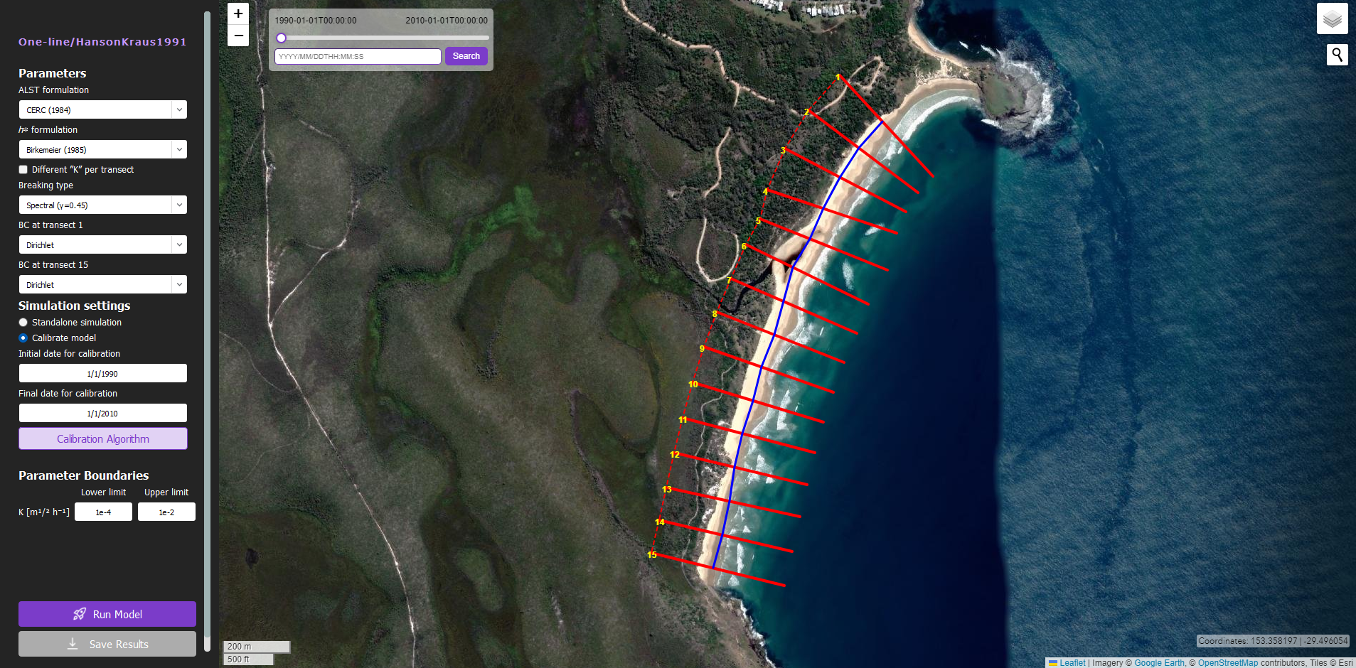 Fig. 3-4-3. Results of simulating the Hanson and Kraus (1991) model for Angourie Back Beach, Australia using the simulaiton settings shown.
Map View: All results are plotted over the same map view shown in Fig. 3-4-2 for easy visualization.
Clickable Transects: Plotted in red, the transects can be individually selected to view the shoreline observations and model results along the transect in plot form. Similar to the other plots generated by IH-SET, the toolbar options can be used to modify and save these plots.
Shoreline Position: Plotted in blue, this line connects the calculated shoreline position at each transect for the selected time stamp to represent the modeled shoreline location.
Adjustable Date-Time: Using the slider or the search bar in the top left, the user can select the time stamp for which the shoreline position is displayed on the map.